
Envelope and maximum theorems#
ECON2125/6012 Lecture 8 Fedor Iskhakov
Announcements & Reminders
Test 3 results and discussion
Thank you for submitting comments to the lecture notes!
Exam is scheduled to Monday, 6 November 9:00 to 12:15, multiple rooms
Plan for this lecture
Correspondences and continuity
The maximum theorem
Envelope theorem
Supplementary reading:
Simon & Blume: 19.1, 19.2
Sundaram: chapter 9, 5.2.3
Parametric continuity#
Value function and parameters of optimization problems#
Let’s start with recalling the definition of a general optimization problem
Definition
The general form of the optimization problem is
where:
\(f(x,\theta) \colon \mathbb{R}^N \times \mathbb{R}^K \to \mathbb{R}\) is an objective function
\(x \in \mathbb{R}^N\) are decision/choice variables
\(\theta \in \mathbb{R}^K\) are parameters
\(g_i(x,\theta) = 0, \; i\in\{1,\dots,I\}\) where \(g_i \colon \mathbb{R}^N \times \mathbb{R}^K \to \mathbb{R}\), are equality constraints
\(h_j(x,\theta) \le 0, \; j\in\{1,\dots,J\}\) where \(h_j \colon \mathbb{R}^N \times \mathbb{R}^K \to \mathbb{R}\), are inequality constraints
\(V(\theta) \colon \mathbb{R}^K \to \mathbb{R}\) is a value function
This lecture focuses on the value function in the optimization problem \(V(\theta)\), and how it depends on the parameters \(\theta\).
In economics we are interested how the optimized behavior changes when the circumstances of the decision-making process change
income/budget/wealth changes
intertemporal effects of changes in other time periods
We would like to establish the properties of the value function \(V(\theta)\):
continuity \(\rightarrow\) The maximum theorem
changes/derivative (if differentiable) \(\rightarrow\) Envelope theorem
monotonicity \(\rightarrow\) Supermodularity and increasing differences (not covered here, see Sundaram ch.10)
Main idea for the maximum theorem
When the components of the optimization problem \(f(x,\theta)\), \(g_i(x,\theta)\) and \(h_j(x,\theta)\) are continuous, then the value function \(V(\theta)\) is also continuous, in certain sense
We need to accurately define the notion of continuity for all components of the optimization problem
objective function
constraints \(\leftrightarrow\) admissible set
Denote the admissible set \(\mathcal{D}(\theta)\)
In solving the optimization problem we are not only interested in the attainable optimal value \(V(\theta)\), but also in the set of maximizers/minimizers \(\mathcal{D}^\star(\theta)\) corresponding to each parameter value \(\theta\)
Definition
We will refer to the pair
as the solution of the optimization problem
where
Correspondences#
Note that the mappings of \(\theta\) to \(\mathcal{D}(\theta)\) or \(\mathcal{D}^\star(\theta)\) are not functions because both \(\mathcal{D}(\theta)\) and often \(\mathcal{D}^\star(\theta)\) have multiple elements for a given \(\theta\)
Definition
A correspondence (set-valued function) is a map that associates elements of its domain to sets of elements in its range, i.e.
where \(P(\mathbb{R}^N)\) denotes the power set of \(\mathbb{R}^N\), i.e. the set of all subsets of \(\mathbb{R}^N\). It can also be denoted as \(2^{\mathbb{R}^N}\).
Example
Let correspondence \(\Phi\) be defined as
Example
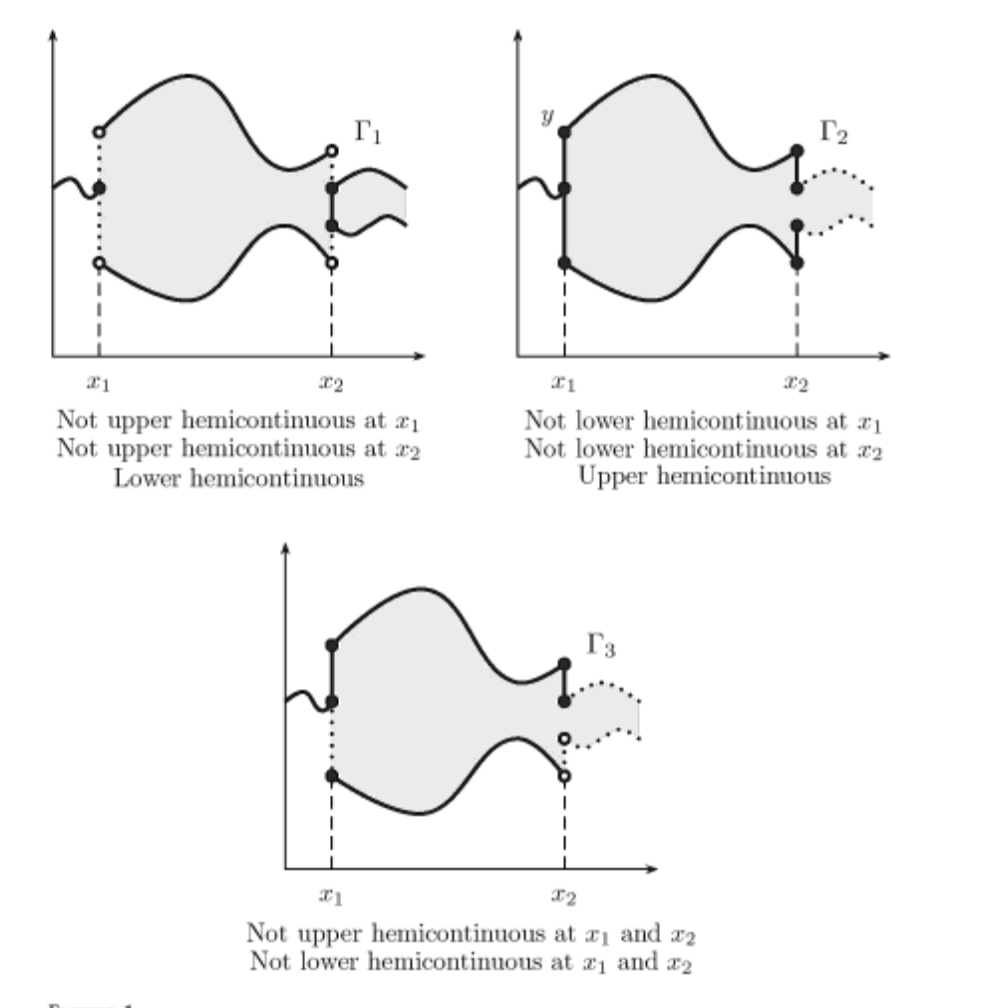
Fig. 106 Examples of correspondences (for labels see below)#
Correspondences are classified by the properties of the sets they output:
open-valued correspondences
closed-valued correspondences
non-empty-valued correspondences
bounded-valued correspondences
convex-valued correspondences
compact-valued correspondences
finite-valued correspondences
singleton-valued correspondences (functions?)
Continuity of correspondences#
Recall the definition of the continuous function
Definition
Function \(f \colon A \subset \mathbb{R}^n \to \mathbb{R}^m\) is called continuous at \({\bf x} \in A\) if as \(n \to \infty\) for every converging to \({\bf x}\) sequence
The equivalent definition of continuity relies on the the open epsilon-balls
Fact
A function \(f \colon A \subset \mathbb{R}^n \to \mathbb{R}^m\) is continuous at \({\bf x} \in A\) if and only if for every \(\epsilon >0\) there is a \(\delta>0\) such that
Proof
Omitted here, but see https://www.u.arizona.edu/~mwalker/MathCamp2020/ContinuousFunctions.pdf
Thinking of the definition of limit stated in terms of open epsilon-balls, it is not hard to see the equivalence result
Generalization to correspondences is not straightforward because \(\in\) operation does not convert to the set-valued case immediately:
can be replaced by set inclusion \(\subset\)
can be represented by non-empty intersection \(\bar{\cap}\), i.e. \(A \bar{\cap} B \iff A \cap B \ne \emptyset \)
Namely, the condition in the definition above can be replaced with either
\({\bf x}' \in B_\delta({\bf x}) \implies f({\bf x}') \subset B_\epsilon(f({\bf x}))\), or
\({\bf x}' \in B_\delta({\bf x}) \ne \emptyset \implies f({\bf x}') \cap B_\epsilon(f({\bf x})) \ne \emptyset\)
Definition
Correspondence \(\gamma \colon X \to 2^Y\) is called upper hemi-continuous (uhc) at \({\bf x} \in X\) if for every open set \(V\) containing \(f({\bf x})\), i.e. \(f({\bf x}) \subset V\), there is an open set \(U\) such that
Correspondence \(\gamma \colon X \to 2^Y\) is called lower hemi-continuous (lhc) at \({\bf x} \in X\) if for every open set \(V\) intersecting with \(f({\bf x})\), i.e. \(f({\bf x}) \cap V \ne \emptyset\), there is an open set \(U\) such that
Definition
A corresponse is called continous if it is both upper and lower hemi-continuous
Note
Semi-continuity is a special notion of continuity for functions, and may be used as equivalent to hemi-continuity for correspondences
Examples, examples, examples (whiteboard)
Fact
Constant correspondences are both uhc and lhc
Note
For closed-valued correspondences, a good rule of thumb for determining hemi-continuity at \({\bf x}\) is:
if moving “a little amount” away from \({\bf x}\) no new points are “discontinuously/suddenly” appear outside of \(f({\bf x})\), \(f\) is uhc
if moving “a little amount” away from \({\bf x}\) no points “suddenly” disappear from \(f({\bf x})\), \(f\) is lhc
The statement of the maximum theorem#
Extremely useful in many fields of economics:
demand (consumer) theory
theory of the firm: supply of products, demand for inputs
theory of economic growth
game theory and industrial relations
The maximum theorem
Let \(f(x,\theta) \colon \mathbb{R}^N \times \mathbb{R}^K \to \mathbb{R}\) be a continuous function, and \(\mathcal{D}(\theta)\) be a compact-valued continuous correspondence. Then the value function \(V(\theta)\) is continuous on \(\mathbb{R}^K\) and \(\mathcal{D}^\star(\theta)\) is a compact-valued upper hemi-continuous correspondence on \(\Theta\)
In other words, continuity of the fundamentals of the optimization problem are inherited by the value function, but not to the full extent (continuity \(\to\) hemi-continuity)
Maximum theorem under convexity
Let \(f(x,\theta) \colon \mathbb{R}^N \times \mathbb{R}^K \to \mathbb{R}\) be a continuous function, and \(\mathcal{D}(\theta)\) be a compact-valued continuous correspondence. Then:
The value function \(V(\theta)\) is continuous on \(\mathbb{R}^K\) and \(\mathcal{D}^\star(\theta)\) is a compact-valued upper hemi-continuous correspondence on \(\Theta\) (as before)
If \(f(x,\theta)\) is concave in \(x\) and \(\mathcal{D}(\theta)\) is convex-valued for every \(\theta\), then \(\mathcal{D}^\star(\theta)\) is a convex-valued.
If concavity of \(f(x,\theta)\) is strict, then \(\mathcal{D}^\star(\theta)\) is a singleton-valued upper hemi-continuous correspondence, hence a continuous functionIf \(f\) is concave in \((x,\theta)\) and the graph of \(\mathcal{D}(\theta)\) is convex, in addition to the above the value function \(V(\theta)\) is concave. Under strict concavity \(V(\theta)\) is also strictly concave.
Definition
The graph of a correspondence \(\gamma \colon X \to 2^Y\) is defined as the set \(\{(x,y) \in X \times Y \colon y \in f(x)\}\)
Consider a special case for when the optimizer is unique for each \(\theta\)
Fact
A single-valued correspondence that is hemi-continuous (either uhc or lhc) is continuous when viewed as a function. Conversely, every continuous function, when viewed as a single-valued correspondence, is both uhc and lhc.
In this case the upper semi-continuity, lower semi-continuity coincide with the “usual” continuity
Example
Budget correspondence in the two goods consumer optimization problem. Assuming \(p_1>0,\, p_2>0,\, m>0\), the budget correspondence can be defined as
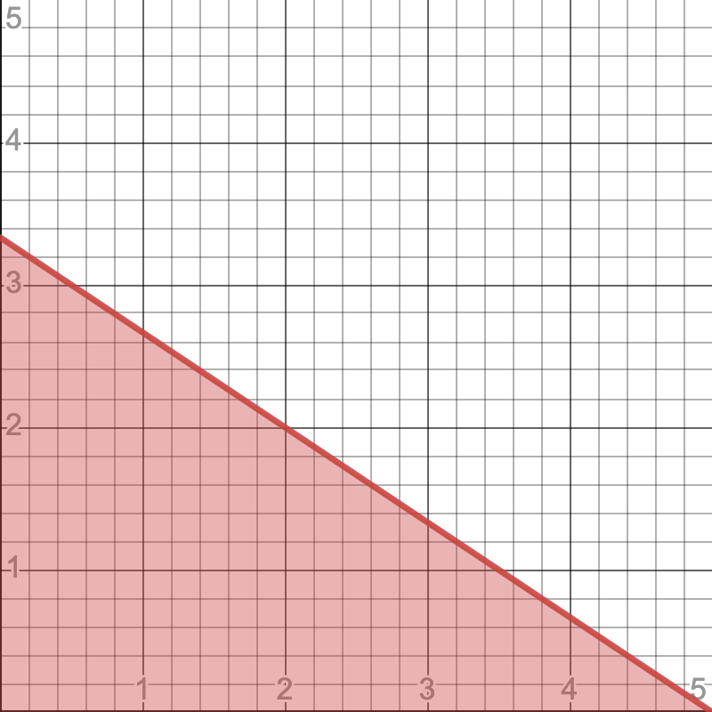
See online animation
Fact
Budget correspondence \(\beta\) defined above is both uhc and lhc, and therefore continuous
Example
Maximization of log utility subject to budget constraint
\(p_i\) is the price of good \(i\), \(p_i>0\)
\(m\) is the budget, assumed non-negative
\(\alpha>0\), \(\beta>0\)
\(x_1 \geq 0, \; x_2 \geq 0\), can show that these constraints never bind
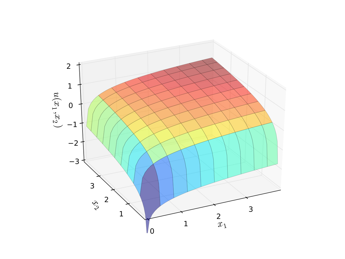
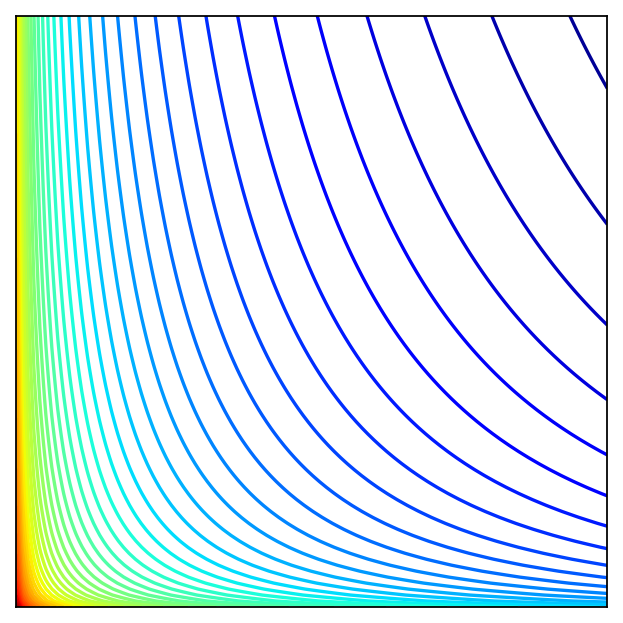
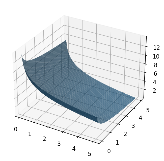
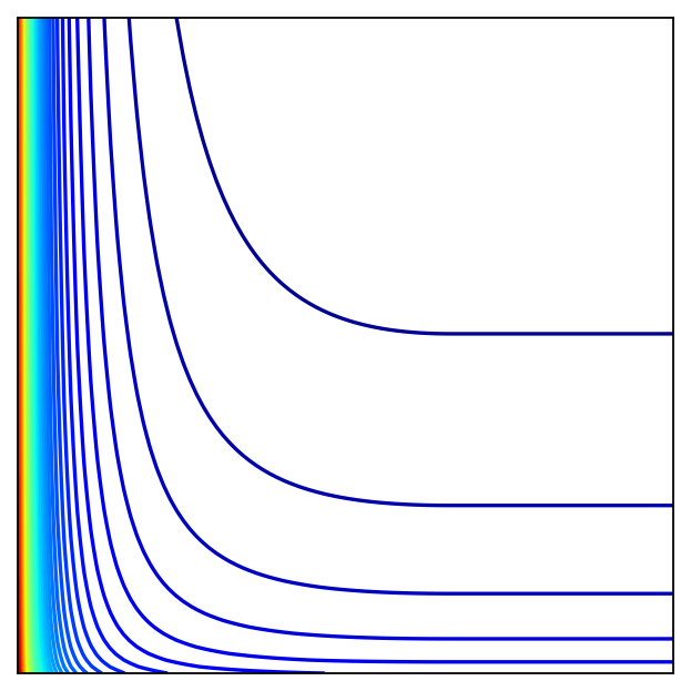
Fig. 107 Log utility with \(\alpha=0.4\), \(\beta=0.5\)#
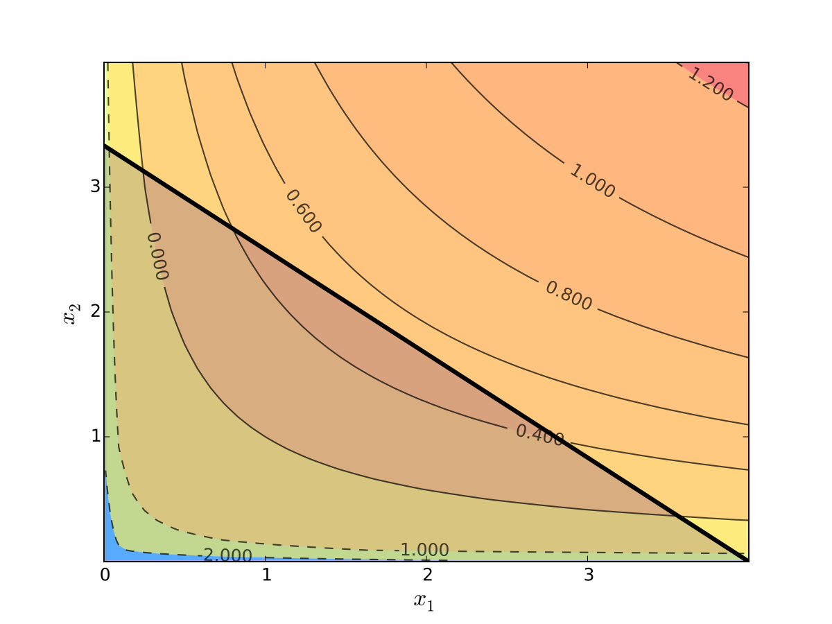
Fig. 108 Utility max for \(p_1=1\), \(p_2 = 1.2\), \(m=4\), \(\alpha=0.4\), \(\beta=0.5\)#
The maximizer according to the FOC conditions and verified with SOC (see lecture 8) is
Applying the maximum theorem:
Objective function is continuous in all arguments
Constrained set is compact for all parameters (as they are defined)
Budget correspondence is continuous
Therefore the theorem applies and we have: the value function is continuous in all parameters, and the set of maximizers is upper hemi-continuous.
Moreover, we can show that the utility function is strictly concave for all parameters, therefore the clause 2 of the maximum theorem under convexity applies, and the set of maximizers is a singleton-valued correspondence, i.e. a function. We have already found it above.
We can verify that the value function is indeed continuous by plugging the maximizer back into the objective function
Question
Can \(\alpha\) and \(\beta\) be also considered as parameters in the previous analysis?
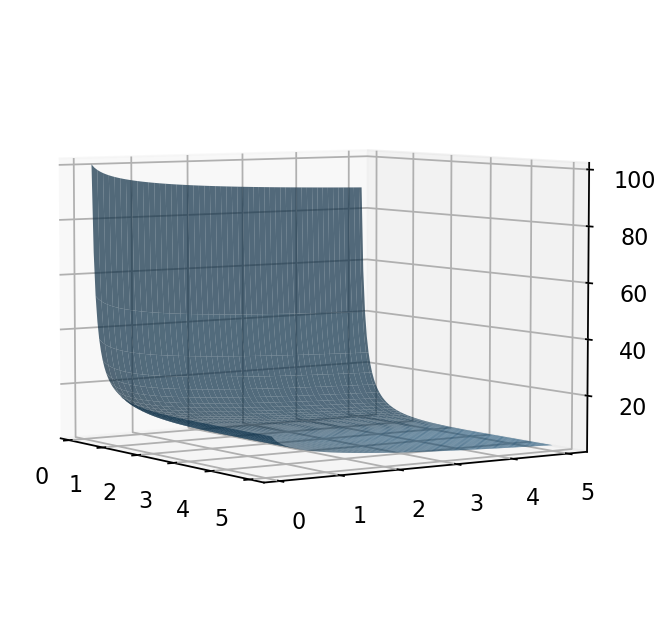
For the numerical example set \(\alpha = 2\), \(\beta = 1\), \(m = 10\), and let \(p_1\) and \(p_2\) vary
Show code cell source
import numpy as np
import matplotlib.pyplot as plt
from mpl_toolkits.mplot3d import Axes3D
from matplotlib import cm

alpha = 2
beta = 1
m = 10
f = lambda x: alpha * np.log( alpha * m / ( (alpha+beta)*x[0] )) + beta * np.log( beta * m / ( (alpha+beta)*x[1] ))

lb,ub = .05,5

x = y = np.linspace(lb,ub, 100)
X, Y = np.meshgrid(x, y)
zs = np.array([f((x,y)) for x,y in zip(np.ravel(X), np.ravel(Y))])
Z = zs.reshape(X.shape)

fig = plt.figure(dpi=160)
ax2 = fig.add_subplot(111)
ax2.set_aspect('equal', 'box')
ax2.contour(X, Y, Z, 50,
            cmap=cm.jet)
plt.setp(ax2, xticks=[],yticks=[])

fig = plt.figure(dpi=160)
ax3 = fig.add_subplot(111, projection='3d')
ax3.plot_surface(X, Y, Z,
            rstride=2,
            cstride=2,
            alpha=0.7,
            linewidth=0.25)

plt.show()
Show code cell source
alpha = 2
beta = 1
m = 10
# f = lambda x: alpha * np.log( alpha * m / ( (alpha+beta)*x[0] )) + beta * np.log( beta * m / ( (alpha+beta)*x[1] ))
f1 = lambda x: alpha * m / ( (alpha+beta)*x)
f2 = lambda x: beta * m / ( (alpha+beta)*x)

lb,ub = .5,5
x = np.linspace(lb,ub, 100)

fig = plt.figure(dpi=160)
ax = fig.add_subplot(111)
ax.plot(x,f1(x),label=r"$x_1^\star(p_1)$")
ax.plot(x,f2(x),label=r"$x_2^\star(p_2)$")
plt.legend(loc='upper right', frameon=False)
plt.show()
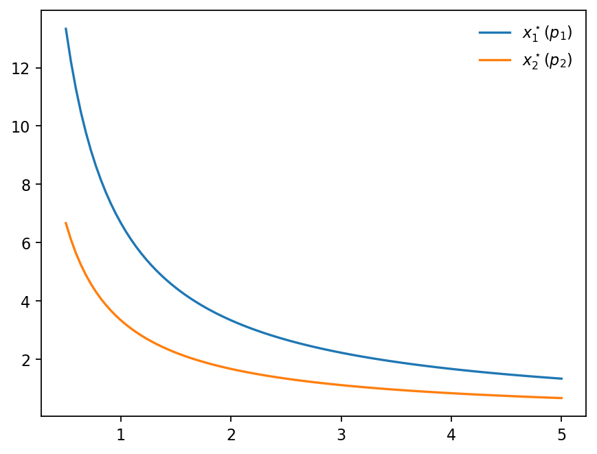
Fig. 111 Optimal choice of \(x_1\) and \(x_2\) as function of prices \(p_1\) and \(p_2\) (aka demand curve)#
Example
Maximization of log-linear utility subject to budget constraint
\(p_i\) is the price of good \(i\), assumed non-negative
\(m\) is the budget, assumed non-negative
\(\alpha>0\), \(\beta>0\)
Form the Lagrangian with 3 inequality constraints (have to flip the sign for non-negativity to stay within the general formulation)
The necessary KKT conditions are given by the following system of equations
The KKT conditions can be solved systematically by considering all combinations of the multipliers. The two cases where the system is consistent give the solution
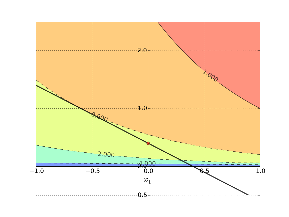
Fig. 112 Corner solution#
Applying the maximum theorem:
Objective function is continuous in all arguments
Constrained set is compact for all parameters (as they are defined)
Budget correspondence is continuous
Therefore the theorem applies and we have: the value function is continuous in all parameters, and the set of maximizers is upper hemi-continuous.
Moreover, we can show that the utility function is strictly concave for all parameters, therefore the clause 2 of the maximum theorem under convexity applies, and the set of maximizers is a singleton-valued correspondence, i.e. a function. We have already found it above.
We can verify that the value function is indeed continuous by plugging the maximizer back into the objective function
Show code cell source
import numpy as np
import matplotlib.pyplot as plt
from mpl_toolkits.mplot3d import Axes3D
from matplotlib import cm

alpha = 1
beta = 3
m = 10
cond = lambda p1: p1/m <= alpha/beta
f = lambda p: cond(p[0])*( alpha * m / p[0] - beta + beta * np.log( beta * p[0] / ( alpha * p[1] )) ) + (1-cond(p[0])) * (beta * np.log( m / p[1] ))

lb,ub = .1,5

x = y = np.linspace(lb,ub, 100)
X, Y = np.meshgrid(x, y)
zs = np.array([f((x,y)) for x,y in zip(np.ravel(X), np.ravel(Y))])
Z = zs.reshape(X.shape)

fig = plt.figure(dpi=160)
ax2 = fig.add_subplot(111)
ax2.set_aspect('equal', 'box')
ax2.contour(X, Y, Z, 50,
            cmap=cm.jet)
plt.setp(ax2, xticks=[],yticks=[])

fig = plt.figure(dpi=160)
ax3 = fig.add_subplot(111, projection='3d')
ax3.plot_surface(X, Y, Z,
            rstride=2,
            cstride=2,
            alpha=0.7,
            linewidth=0.25)
ax3.view_init(elev=5, azim=-34)

plt.show()
Show code cell source
alpha = 1
beta = 3
m = 10
cond = lambda p1: p1/m <= alpha/beta
f1 = lambda x: cond(x)*(m/x - beta/alpha) + (1-cond(x))*0
lb,ub = .5,10
x = np.linspace(lb,ub, 100)
fig = plt.figure(dpi=160)
ax = fig.add_subplot(111)
ax.plot(x,f1(x),label=r"$x_1^\star(p_1)$")
plt.legend(loc='upper right', frameon=False)
plt.show()
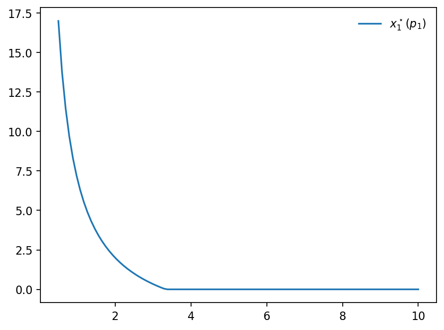
Fig. 115 Optimal choice of \(x_1\) as a function of \(p_1\) (aka demand curve)#
Show code cell source
alpha = 1
beta = 3
m = 10
cond = lambda p1: p1/m <= alpha/beta
f = lambda p: cond(p[0])*( beta * p[0] / (alpha *p[1]) ) + (1-cond(p[0])) * (m / p[1])
lb,ub = .5,5
x = y = np.linspace(lb,ub, 100)
X, Y = np.meshgrid(x, y)
zs = np.array([f((x,y)) for x,y in zip(np.ravel(X), np.ravel(Y))])
Z = zs.reshape(X.shape)
fig = plt.figure(dpi=160)
ax3 = fig.add_subplot(111, projection='3d')
ax3.plot_surface(X, Y, Z,
            rstride=2,
            cstride=2,
            alpha=0.7,
            linewidth=0.25)
plt.setp(ax3,xticks=[],yticks=[],zticks=[])
ax3.view_init(elev=22, azim=123)
plt.show()
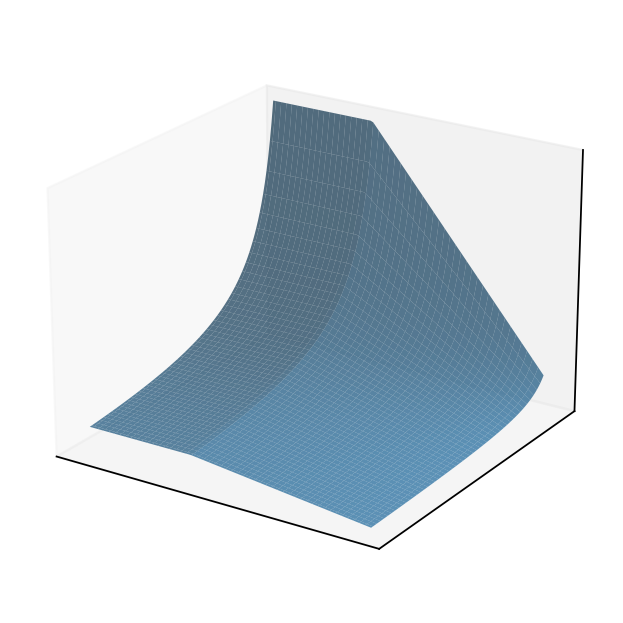
Fig. 116 Optimal choice of \(x_2\) as a function of \((p_1,p_2)\) (aka demand curve)#
Envelope theorems#
Next step after continuity – differentiability of the value function \(V(\theta)\) and the marginal effect of relaxing the constraint (derivatives!)
Let’s start with an unconstrained optimization problem
where:
\(f(x,\theta) \colon \mathbb{R}^N \times \mathbb{R}^K \to \mathbb{R}\) is an objective function
\(x \in \mathbb{R}^N\) are decision/choice variables
\(\theta \in \mathbb{R}^K\) are parameters
\(V(\theta) \colon \mathbb{R}^K \to \mathbb{R}\) is a value function
Envelope theorem for unconstrained problems
Let \(f(x,\theta) \colon \mathbb{R}^N \times \mathbb{R}^K \to \mathbb{R}\) be a differentiable function, and \(x^\star(\theta)\) be the maximizer of \(f(x,\theta)\) for every \(\theta\). Suppose that \(x^\star(\theta)\) is differentiable function itself. Then the value function of the problem \(V(\theta) = f\big(x^\star(\theta),\theta)\) is differentiable w.r.t. \(\theta\) and
In other words, the marginal changes in the value function are given by the partial derivative of the objective function evaluated at the maximizer.
Proof
Exercise
Note
When \(K=1\), so that \(\theta\) is a scalar, the envelope theorem can be written as
so that the meaning is carried only by the derivative sign change
Example
Consider \(f(x,a) = -x^2 +2ax +4a^2 \to \max_x\).
What is the (approximate) effect of a unit increase in \(a\) on the attained maximum?
FOC: \(-2x+2a=0\), giving \(x^\star(a) = a\).
So, \(V(a) = f(a,a) = 5a^2\), and \(V'(a)=10a\). The value increases at a rate of \(10a\) per unit increase in \(a\).
Using the envelope theorem, we could go directly to
Envelope theorem for constrained problems
Consider an equality constrained optimization problem
where:
\(f(x,\theta) \colon \mathbb{R}^N \times \mathbb{R}^K \to \mathbb{R}\) is an objective function
\(x \in \mathbb{R}^N\) are decision/choice variables
\(\theta \in \mathbb{R}^K\) are parameters
\(g_i(x,\theta) = 0, \; i\in\{1,\dots,I\}\) where \(g_i \colon \mathbb{R}^N \times \mathbb{R}^K \to \mathbb{R}\), are equality constraints
\(V(\theta) \colon \mathbb{R}^K \to \mathbb{R}\) is a value function
Assume that the maximizer correspondence \(\mathcal{D}^\star(\theta) = \mathrm{arg}\max f(x,\theta)\) is single-valued and can be represented by the function \(x^\star(\theta) \colon \mathbb{R}^K \to \mathbb{R}^N\), with the corresponding Lagrange multipliers \(\lambda^\star(\theta) \colon \mathbb{R}^K \to \mathbb{R}^K\).
Assume that both \(x^\star(\theta)\) and \(\lambda^\star(\theta)\) are differentiable, and that the constraint qualification assumption holds. Then
where \(\mathcal{L}(x,\lambda,\theta)\) is the Lagrangian of the problem.
Proof
Exercise
Note
What about the inequality constraints?
Well, if the solution is interior and none of the constrains are binding, the unconstrained version of the envelope theorem applies. If any of the constrains are binding, their combination can be represented as a set of equality constraint, and the constrained version of the envelope theorem applies. Care needs to be taken to avoid the changes in the parameter that lead to a switch in the binding constraints. Such points are most likely non-differentiable, and the envelope theorem does not apply there at all!
Example
Back to the log utility case
The Lagrangain is
Solution is
Value function is
We can verify the Envelope theorem by noting that direct differentiation gives
And applying the envelope theorem we have
Lagrange multiplyers as shadow prices#
In the equality constrained optimization problem, the Lagrange multiplier \(\lambda_i\) can be interpreted as the shadow price of the constraint \(g_i(x,\theta) = a\), i.e. the change in the value function resulting from a change in parameter \(a\), in other words relaxing the constraint \(g_i(x,\theta) = 0\).
Exercise: prove this statement