Elements of linear algebra#
ECON2125/6012 Lecture 5
Fedor Iskhakov
Announcements & Reminders
Tests due last night: feedback soon
This lecture is recorded
Next week we return to the class
Plan for this lecture
Review of some concepts in linear algebra
Vector spaces
Linear combinations, span, linear independence
Linear subspaces, bases and dimension
Linear maps and independence
Linear equations
Basic operations with matrices
Square and invertible matrices
Determinant
Quadratic forms
Eigenvalues and diagonalization
Symmetric matrices
Positive and negative definiteness
Supplementary reading:
Stachurski: 2.1, 3.1, 3.2
Simon & Blume: 6.1, 6.2, 10.1, 10.2, 10.3, 10.4, 10.5, 10.6, 11, 16, 23.7, 23.8
Sundaram: 1.3, Appendix C.1, C.2
Intro to Linear Algebra#
Linear algebra is used to study linear models
Foundational for many disciplines related to economics
Economic theory
Econometrics and statistics
Finance
Operations research
Example of linear model
Equilibrium in a single market with price \(p\)
What price \(p\) clears the market, and at what quantity \(q = q_s = q_d\)?
Here \(a, b, c, d\) are the model parameters or coefficients
Treated as fixed for a single computation but might vary between computations to better fit the data
Example
Determination of income
Question: discuss what the variables are
Solve for \(Y\) as a function of \(I\) and \(G\)
Bigger, more complex systems found in problems related to
Regression and forecasting
Portfolio analysis
Ranking systems
Etc., etc. — any number of applications
Definition
A general system of equations can be written as
Typically
the \(a_{ij}\) and \(b_i\) are exogenous / given / parameters
the values \(x_j\) are endogenous
Key question: What values of \(x_1, \ldots, x_K\) solve this system?
More often we write the system in matrix form
or
Notice bold font to indicate that the variables are vectors.
Let’s solve this system on a computer:
import numpy as np
from scipy.linalg import solve
A = [[0, 2, 4],
     [1, 4, 8],
     [0, 3, 7]]
b = (1, 2, 0)
A, b = np.asarray(A), np.asarray(b)
x=solve(A, b)
print(f'Solutions is x={x}')
Solutions is x=[-1.77635684e-15 3.50000000e+00 -1.50000000e+00]
This tells us that the solution is \(x = (0. , 3.5, -1.5)\)
That is,
The usual question: if computers can do it so easily — what do we need to study for?
But now let’s try this similar looking problem
Question: what changed?
import numpy as np
from scipy.linalg import solve
A = [[0, 2, 4],
     [1, 4, 8],
     [0, 3, 6]]
b = (1, 2, 0)
A, b = np.asarray(A), np.asarray(b)
x=solve(A, b)
print(f'Solutions is x={x}')
Solutions is x=[ 0.00000000e+00 -9.00719925e+15 4.50359963e+15]
/var/folders/5d/cjhpvdlx7lg8zt1ypw5fcyy40000gn/T/ipykernel_77087/3978225594.py:8: LinAlgWarning: Ill-conditioned matrix (rcond=4.11194e-18): result may not be accurate.
  x=solve(A, b)
This is the output that we get:
LinAlgWarning: Ill-conditioned matrix
What does this mean?
How can we fix it?
We still need to understand the concepts after all!
Vector Space#
Recall that \(\mathbb{R}^N := \) set of all \(N\)-vectors
Definition
An \(N\)-vector \({\bf x}\) is a tuple of \(N\) real numbers:
We typically think of vectors as columns, and can write \({\bf x}\) vertically, like so:
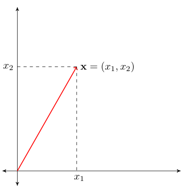
Fig. 42 Visualization of vector \({\bf x}\) in \(\mathbb{R}^2\)#
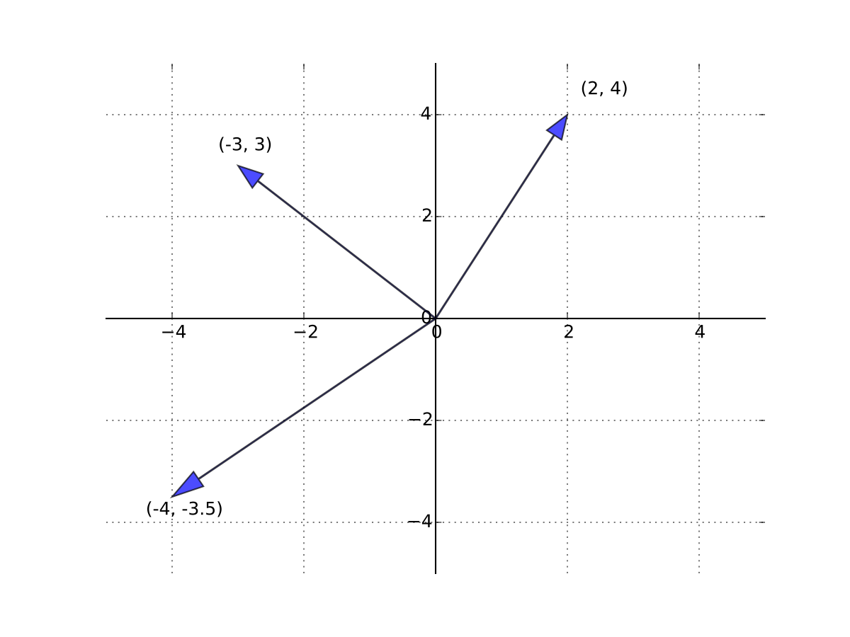
Fig. 43 Three vectors in \(\mathbb{R}^2\)#
The vector of ones will be denoted \({\bf 1}\)
Vector of zeros will be denoted \({\bf 0}\)
Linear Operations#
Two fundamental algebraic operations:
Vector addition
Scalar multiplication
Definition
Sum of \({\bf x} \in \mathbb{R}^N\) and \({\bf y} \in \mathbb{R}^N\) defined by
Example
Example
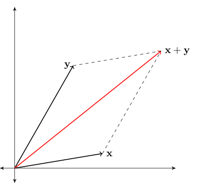
Fig. 44 Vector addition#
Definition
Scalar product of \(\alpha \in \mathbb{R}\) and \({\bf x} \in \mathbb{R}^N\) defined by
Example
Example
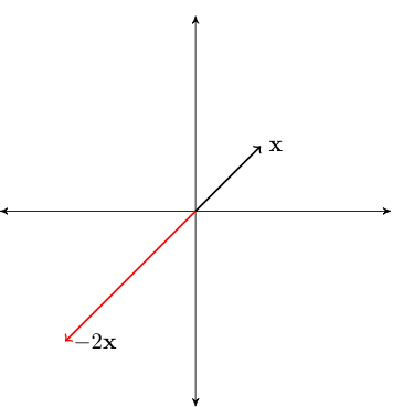
Fig. 45 Scalar multiplication#
Subtraction performed element by element, analogous to addition
Def can be given in terms of addition and scalar multiplication:
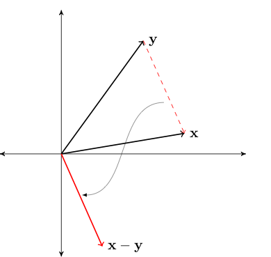
Fig. 46 Difference between vectors#
Incidentally, most high level numerical libraries treat vector addition and scalar multiplication in the same way — element-wise
import numpy as np
x = np.array((2, 4, 6))
y = np.array((10, 10, 10))
print(x + y) # Vector addition

x = np.array([12, 14, 16])
print(2 * x) # Scalar multiplication
[12 14 16]
[24 28 32]
Definition
A linear combination of vectors \({\bf x}_1,\ldots, {\bf x}_K\) in \(\mathbb{R}^N\) is a vector
where \(\alpha_1,\ldots, \alpha_K\) are scalars
Example
Inner Product#
Definition
The inner product of two vectors \({\bf x}\) and \({\bf y}\) in \(\mathbb{R}^N\) is
The notation \(\bullet '\) flips the vector from column-vector to row-vector, this will make sense when we talk later about matrices for which vectors are special case.
Example
\({\bf x} = (2, 3)\) and \({\bf y} = (-1, 1)\) implies that
Example
\({\bf x} = \tfrac{1}{N} {\bf 1}\) and \({\bf y} = (y_1, \ldots, y_N)\) implies
import numpy as np
x = np.array((1, 2, 3, 4))
y = np.array((2, 4, 6, 8))
print('Product =',x * y)
print('Inner product =',np.sum(x * y))
print('Inner product =',x @ y)
Product = [ 2  8 18 32]
Inner product = 60
Inner product = 60
Fact
For any \(\alpha, \beta \in \mathbb{R}\) and any \({\bf x}, {\bf y} \in \mathbb{R}^N\), the following statements are true:
\({\bf x}' {\bf y} = {\bf y}' {\bf x}\)
\((\alpha {\bf x})' (\beta {\bf y}) = \alpha \beta ({\bf x}' {\bf y})\)
\({\bf x}' ({\bf y} + {\bf z}) = {\bf x}' {\bf y} + {\bf x}' {\bf z}\)
For example, item 2 is true because
Exercise: Use above rules to show that \((\alpha {\bf y} + \beta {\bf z})'{\bf x} = \alpha {\bf x}' {\bf y} + \beta {\bf x}' {\bf z}\)
The next result is a generalization
Fact
Inner products of linear combinations satisfy
(Reminder about) Norms and Distance#
The (Euclidean) norm of \({\bf x} \in \mathbb{R}^N\) is defined as
Interpretation:
\(\| {\bf x} \|\) represents the ``length’’ of \({\bf x}\)
\(\| {\bf x} - {\bf y} \|\) represents distance between \({\bf x}\) and \({\bf y}\)
Fig. 47 Length of red line \(= \sqrt{x_1^2 + x_2^2} =: \|{\bf x}\|\)#
\(\| {\bf x} - {\bf y} \|\) represents distance between \({\bf x}\) and \({\bf y}\)
Fact
For any \(\alpha \in \mathbb{R}\) and any \({\bf x}, {\bf y} \in \mathbb{R}^N\), the following statements are true:
\(\| {\bf x} \| \geq 0\) and \(\| {\bf x} \| = 0\) if and only if \({\bf x} = {\bf 0}\)
\(\| \alpha {\bf x} \| = |\alpha| \| {\bf x} \|\)
\(\| {\bf x} + {\bf y} \| \leq \| {\bf x} \| + \| {\bf y} \|\) (triangle inequality)
\(| {\bf x}' {\bf y} | \leq \| {\bf x} \| \| {\bf y} \|\) (Cauchy-Schwarz inequality)
Proof
See the previous lecture
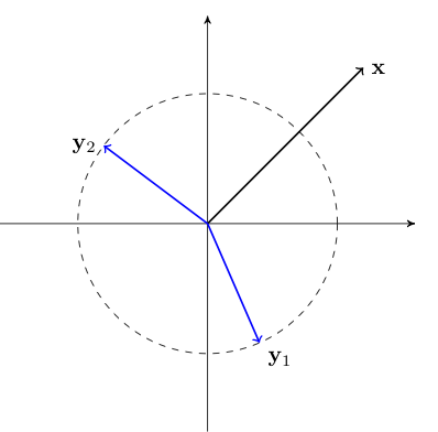
Fact
If \({\bf x} \in \mathbb{R}^N\) is nonzero, then the solution to the optimization problem
is \({\hat{\bf x}} := {\bf x} / \| {\bf x} \|\)
Proof
Fix nonzero \({\bf x} \in \mathbb{R}^N\)
Let \({\hat{\bf x}} := \alpha {\bf x}\) where \(\alpha := 1/\|{\bf x}\|\), that is \({\hat{\bf x}} := {\bf x} / \| {\bf x} \|\)
Evidently \(\| {\hat{\bf x}} \| = 1\) and so it satisfies the constraint
Let’s show that \({\hat{\bf x}}\) is the solution to the optimization problem
Pick any other \({\bf y} \in \mathbb{R}^N\) satisfying \(\| {\bf y} \| = 1\)
We have
The first inequality trivially follows from the definition of the absolute value of a scalar
The second inequality is the application of Cauchy-Schwarz inequality
The third equality takes into account that \(\| {\bf y} \| = 1\)
The forth equality is multiplication of enumerator and denominator by a constant
The fifth equality follows from \(\| {\bf x} \| = \sqrt{{\bf x}'{\bf x}}\)
The sixth equality follows from the properties of the inner product
Taking first and last expression in the above inequality yields that \({\hat{\bf x}}\) is the maximizer, as claimed
Span#
Let \(X \subset \mathbb{R}^N\) be any nonempty set (of points in \(\mathbb{R}^N\), i.e. vectors)
Definition
Set of all possible linear combinations of elements of \(X\) is called the span of \(X\), denoted by \(\mathrm{span}(X)\)
For finite \(X := \{{\bf x}_1,\ldots, {\bf x}_K\}\) the span can be expressed as
We are mainly interested in the span of finite sets…
Example
Let’s start with the span of a singleton
Let \(X = \{ {\bf 1} \} \subset \mathbb{R}^2\), where \({\bf 1} := (1,1)\)
The span of \(X\) is all vectors of the form
Constitutes a line in the plane that passes through
the vector \({\bf 1}\) (set \(\alpha = 1\))
the origin \({\bf 0}\) (set \(\alpha = 0\))
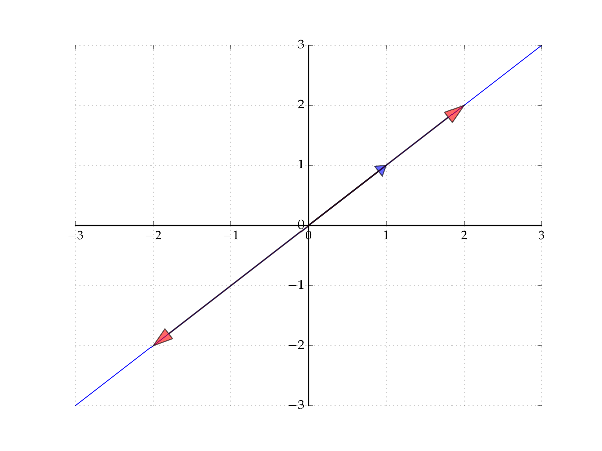
Fig. 48 The span of \({\bf 1} := (1,1)\) in \(\mathbb{R}^2\)#
Example
Let \({\bf x}_1 = (3, 4, 2)\) and let \({\bf x}_2 = (3, -4, 0.4)\)
By definition, the span is all vectors of the form
It turns out to be a plane that passes through
the vector \({\bf x}_1\)
the vector \({\bf x}_2\)
the origin \({\bf 0}\)
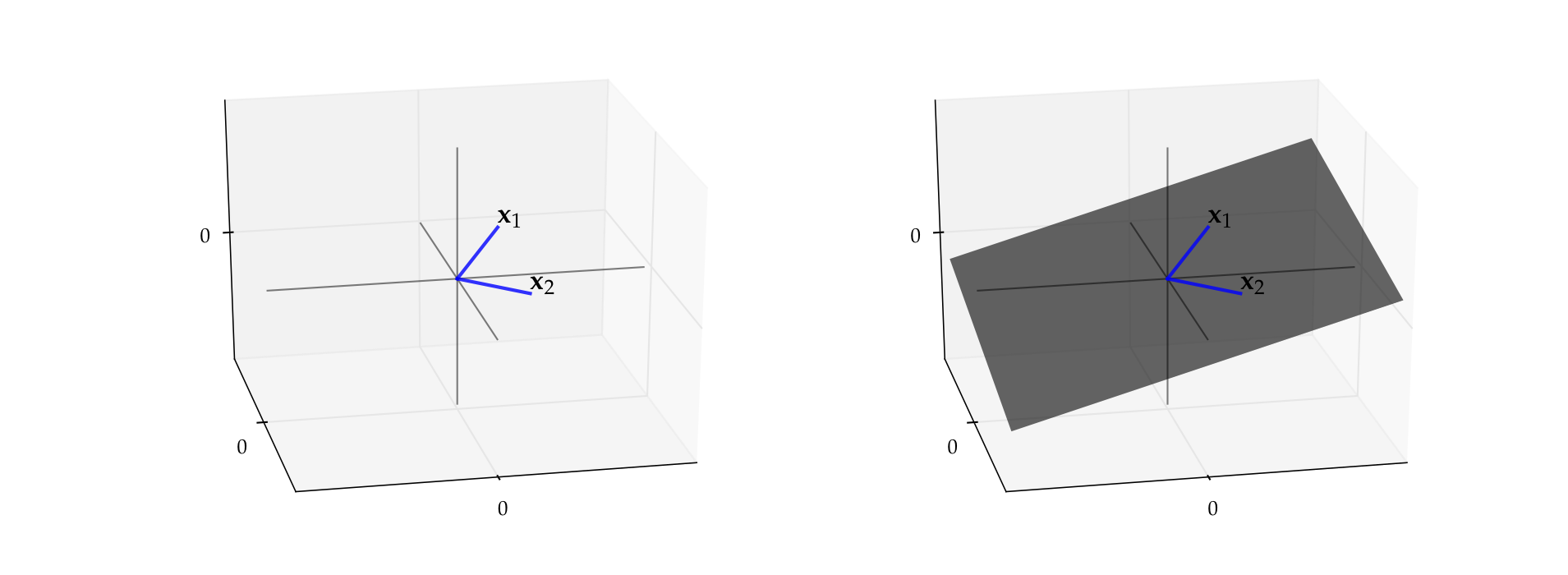
Fig. 49 Span of \({\bf x}_1, {\bf x}_2\)#
Fact
If \(X \subset Y\), then \(\mathrm{span}(X) \subset \mathrm{span}(Y)\)
Proof
Pick any nonempty \(X \subset Y \subset \mathbb{R}^N\)
Letting \({\bf z} \in \mathrm{span}(X)\), we have
Since \(X \subset Y\), each \({\bf x}_k\) is also in \(Y\), giving us
Hence \({\bf z} \in \mathrm{span}(Y)\)
Let \(Y\) be any subset of \(\mathbb{R}^N\), and let \(X:= \{{\bf x}_1,\ldots, {\bf x}_K\}\)
If \(Y \subset \mathrm{span}(X)\), we say that the vectors in \(X\) span the set \(Y\)
Alternatively, we say that \(X\) is a spanning set for \(Y\)
A nice situation: \(Y\) is large but \(X\) is small
\(\implies\) large set \(Y\) ``described’’ by the small number of vectors in \(X\)
Example
Consider the vectors \(\{{\bf e}_1, \ldots, {\bf e}_N\} \subset \mathbb{R}^N\), where
That is, \({\bf e}_n\) has all zeros except for a \(1\) as the \(n\)-th element
Vectors \({\bf e}_1, \ldots, {\bf e}_N\) are called the canonical basis vectors of \(\mathbb{R}^N\)

Fig. 50 Canonical basis vectors in \(\mathbb{R}^2\)#
Fact
The span of \(\{{\bf e}_1, \ldots, {\bf e}_N\}\) is equal to all of \(\mathbb{R}^N\)
Proof
Proof for \(N=2\):
Pick any \({\bf y} \in \mathbb{R}^2\)
We have
Thus, \({\bf y} \in \mathrm{span} \{{\bf e}_1, {\bf e}_2\}\)
Since \({\bf y}\) arbitrary, we have shown that \(\mathrm{span} \{{\bf e}_1, {\bf e}_2\} = \mathbb{R}^2\)
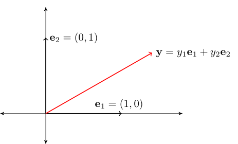
Fig. 51 Canonical basis vectors in \(\mathbb{R}^2\)#
Fact
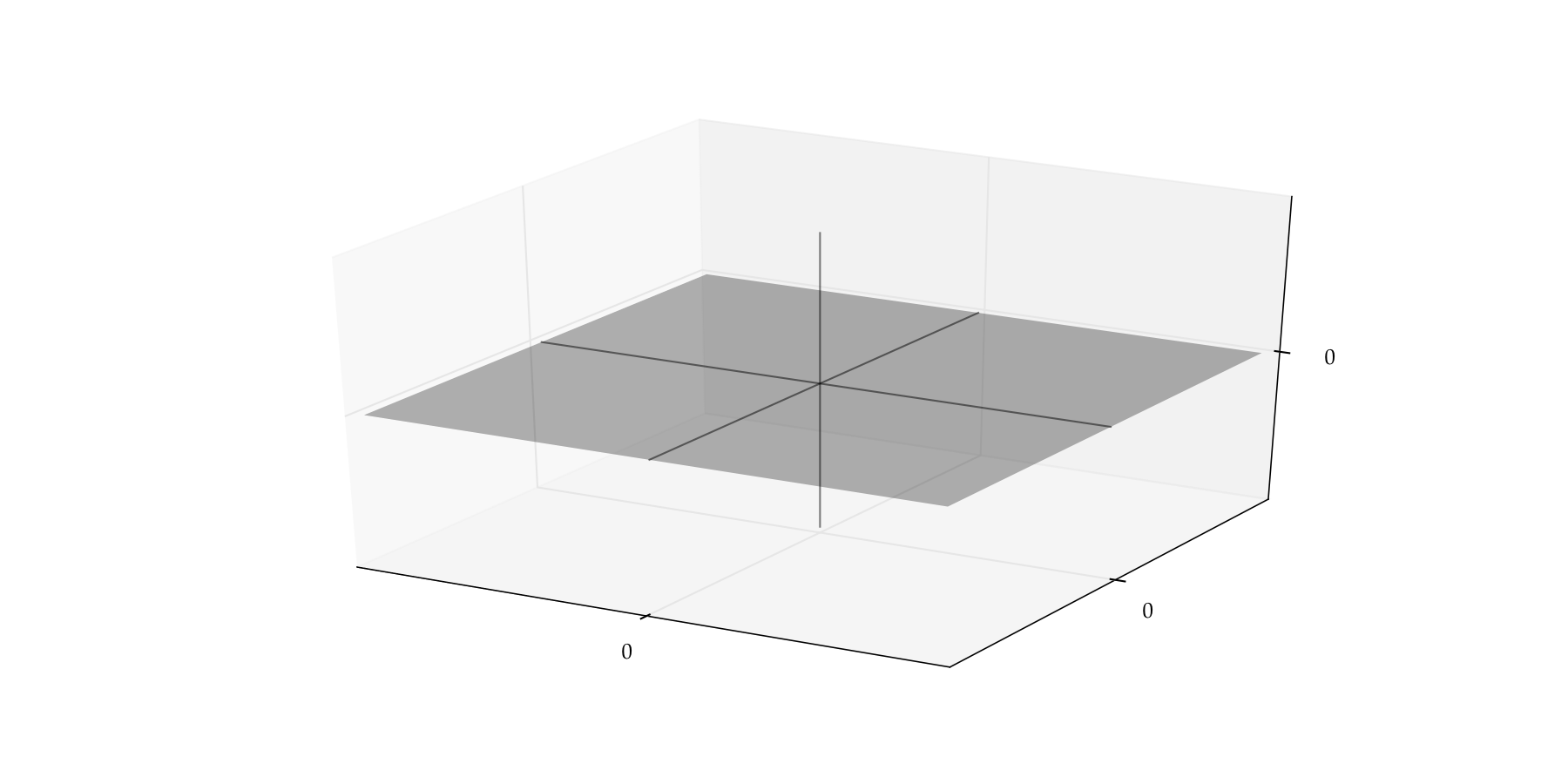
Consider the set
Let \({\bf e}_1\) and \({\bf e}_2\) be the canonical basis vectors in \(\mathbb{R}^3\)
Then \(\mathrm{span}\{{\bf e}_1, {\bf e}_2\} = P\)
Graphically, \(P =\) flat plane in \(\mathbb{R}^3\), where height coordinate \(x_3=0\)
Proof
Let \({\bf x} = (x_1, x_2, 0)\) be any element of \(P\)
We can write \({\bf x}\) as
In other words, \(P \subset \mathrm{span}\{{\bf e}_1, {\bf e}_2\}\)
Conversely (check it) we have \(\mathrm{span}\{{\bf e}_1, {\bf e}_2\} \subset P\)
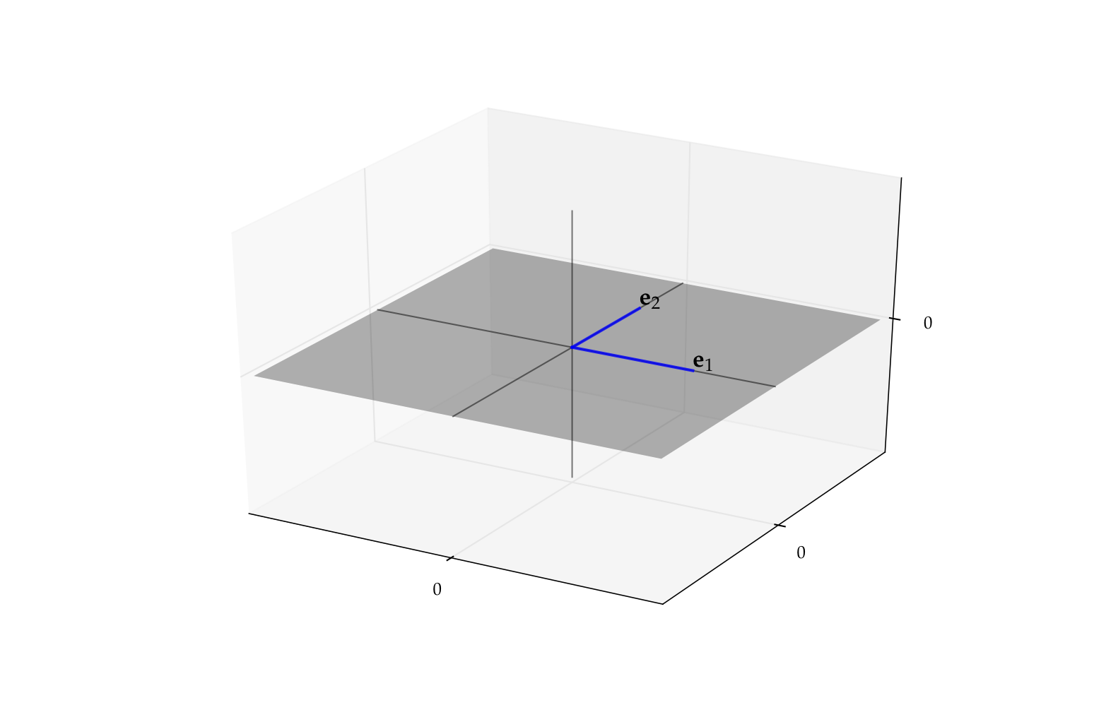
Fig. 52 \(\mathrm{span}\{{\bf e}_1, {\bf e}_2\} = P\)#
Linear Subspaces#
Definition
A nonempty \(S \subset \mathbb{R}^N\) called a linear subspace of \(\mathbb{R}^N\) if
In other words, \(S \subset \mathbb{R}^N\) is “closed” under vector addition and scalar multiplication
Note: Sometimes we just say subspace and drop “linear”
Example
\(\mathbb{R}^N\) itself is a linear subspace of \(\mathbb{R}^N\)
Fact
Fix \({\bf a} \in \mathbb{R}^N\) and let \(A := \{ {\bf x} \in \mathbb{R}^N \colon {\bf a }'{\bf x} = 0 \}\)
The set \(A\) is a linear subspace of \(\mathbb{R}^N\)
Proof
Let \({\bf x}, {\bf y} \in A\) and let \(\alpha, \beta \in \mathbb{R}\)
We must show that \({\bf z} := \alpha {\bf x} + \beta {\bf y} \in A\)
Equivalently, that \({\bf a}' {\bf z} = 0\)
True because
Fact
If \(Z\) is a nonempty subset of \(\mathbb{R}^N\), then \(\mathrm{span}(Z)\) is a linear subspace
Proof
If \({\bf x}, {\bf y} \in \mathrm{span}(Z)\), then \(\exists\) vectors \({\bf z}_k\) in \(Z\) and scalars \(\gamma_k\) and \(\delta_k\) such that
This vector clearly lies in \(\mathrm{span}(Z)\)
Fact
If \(S\) and \(S'\) are two linear subspaces of \(\mathbb{R}^N\), then \(S \cap S'\) is also a linear subspace of \(\mathbb{R}^N\).
Proof
Let \(S\) and \(S'\) be two linear subspaces of \(\mathbb{R}^N\)
Fix \({\bf x}, {\bf y} \in S \cap S'\) and \(\alpha, \beta \in \mathbb{R}\)
We claim that \({\bf z} := \alpha {\bf x} + \beta {\bf y} \in S \cap S'\)
Since \({\bf x}, {\bf y} \in S\) and \(S\) is a linear subspace we have \({\bf z} \in S\)
Since \({\bf x}, {\bf y} \in S'\) and \(S'\) is a linear subspace we have \({\bf z} \in S'\)
Therefore \({\bf z} \in S \cap S'\)
Other examples of linear subspaces
The singleton \(\{{\bf 0}\}\) in \(\mathbb{R}^N\)
Lines through the origin in \(\mathbb{R}^2\) and \(\mathbb{R}^3\)
Planes through the origin in \(\mathbb{R}^3\)
Exercise: Let \(S\) be a linear subspace of \(\mathbb{R}^N\). Show that
\({\bf 0} \in S\)
If \(X \subset S\), then \(\mathrm{span}(X) \subset S\)
\(\mathrm{span}(S) = S\)
Linear Independence#
Important applied questions
When does a set of linear equations have a solution?
When is that solution unique?
When do regression arguments suffer from collinearity?
How can we approximate complex functions parsimoniously?
What is the rank of a matrix?
When is a matrix invertible?
All of these questions closely related to linear independence
Definition
A nonempty collection of vectors \(X := \{{\bf x}_1,\ldots, {\bf x}_K\} \subset \mathbb{R}^N\) is called linearly independent if
As we’ll see, linear independence of a set of vectors determines how large a space they span
Loosely speaking, linearly independent sets span large spaces
Example
Let \({\bf x} := (1, 2)\) and \({\bf y} := (-5, 3)\)
The set \(X = \{{\bf x}, {\bf y}\}\) is linearly independent in \(\mathbb{R}^2\)
Indeed, suppose \(\alpha_1\) and \(\alpha_2\) are scalars with
Equivalently,
Then \(2(5\alpha_2) = 10 \alpha_2 = -3 \alpha_2\), implying \(\alpha_2 = 0\) and hence \(\alpha_1 = 0\)
Example
The set of canonical basis vectors \(\{{\bf e}_1, \ldots, {\bf e}_N\}\) is linearly independent in \(\mathbb{R}^N\)
Proof
Let \(\alpha_1, \ldots, \alpha_N\) be coefficients such that \(\sum_{k=1}^N \alpha_k {\bf e}_k = {\bf 0}\)
Then
In particular, \(\alpha_k = 0\) for all \(k\)
Hence \(\{{\bf e}_1, \ldots, {\bf e}_N\}\) linearly independent
As a first step to better understanding linear independence let’s look at some equivalences
Fact
Take \(X := \{{\bf x}_1,\ldots, {\bf x}_K\} \subset \mathbb{R}^N\). For \(K > 1\) all of following statements are equivalent
\(X\) is linearly independent
No \({\bf x}_i \in X\) can be written as linear combination of the others
\(X_0 \subsetneq X \implies \mathrm{span}(X_0) \subsetneq \mathrm{span}(X)\)
Here \(X_0 \subsetneq X\) means \(X_0 \subset X\) and \(X_0 \ne X\)
We say that \(X_0\) is a proper subset of \(X\)
As an exercise, let’s show that the first two statements are equivalent, first
and the second
We now show that
To show that (1) \(\implies\) (2) let’s suppose to the contrary that
\(\sum_{k=1}^K \alpha_k {\bf x}_k = {\bf 0} \implies \alpha_1 = \cdots = \alpha_K = 0\)
and yet some \({\bf x}_i\) can be written as a linear combination of the other elements of \(X\)
In particular, suppose that
Then, rearranging,
This contradicts 1., and hence (2) holds
To show that (2) \(\implies\) (1) let’s suppose to the contrary that
no \({\bf x}_i\) can be written as a linear combination of others
and yet \(\exists\) \(\alpha_1, \ldots, \alpha_K\) not all zero with \(\alpha_1 {\bf x}_1 + \cdots + \alpha_K {\bf x}_K = {\bf 0}\)
Suppose without loss of generality that \(\alpha_1 \ne 0\) (similar argument works for any \(\alpha_j\))
Then
This contradicts 1., and hence (1) holds.
Let’s show one more part of the proof as an exercise:
Proof
Suppose to the contrary that
\(X\) is linearly independent,
\(X_0 \subsetneq X\) and yet
\(\mathrm{span}(X_0) = \mathrm{span}(X)\)
Let \({\bf x}_j\) be in \(X\) but not \(X_0\)
Since \({\bf x}_j \in \mathrm{span}(X)\), we also have \({\bf x}_j \in \mathrm{span}(X_0)\)
But then \({\bf x}_j\) can be written as a linear combination of the other elements of \(X\)
This contradicts linear independence
Example
Dropping any of the canonical basis vectors reduces span
Consider the \(N=2\) case
We know that \(\mathrm{span} \{{\bf e}_1, {\bf e}_2\} =\) all of \(\mathbb{R}^2\)
Removing either element of \(\mathrm{span} \{{\bf e}_1, {\bf e}_2\}\) reduces the span to a line
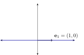
Fig. 53 The span of \(\{{\bf e}_1\}\) alone is the horizonal axis#
Example
As another visual example of linear independence, consider the pair
The span of this pair is a plane in \(\mathbb{R}^3\)
But if we drop either one the span reduces to a line
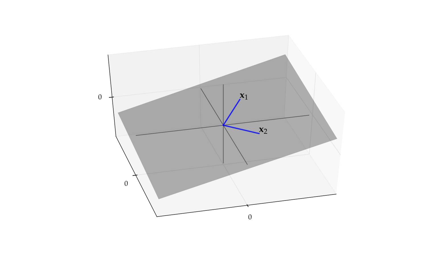
Fig. 54 The span of \(\{{\bf x}_1, {\bf x}_2\}\) is a plane#
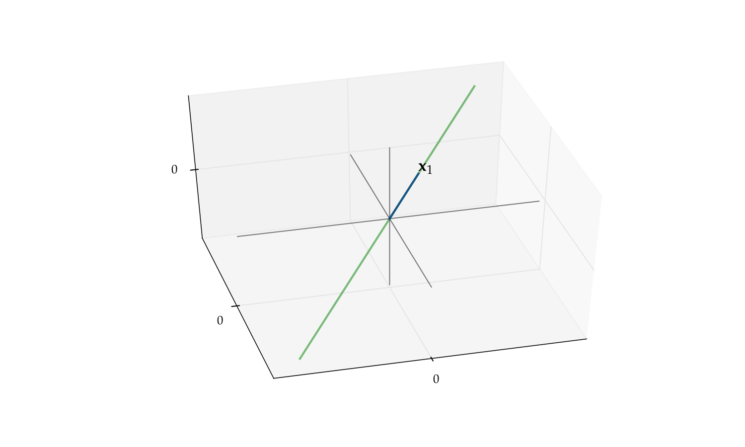
Fig. 55 The span of \(\{{\bf x}_1\}\) alone is a line#
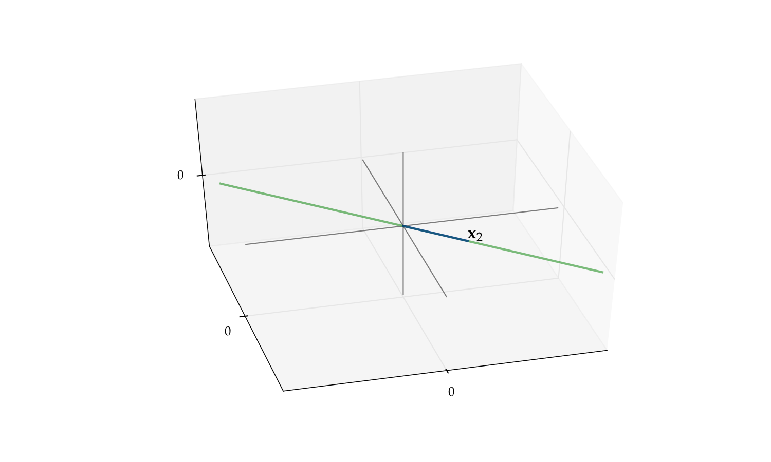
Fig. 56 The span of \(\{{\bf x}_2\}\) alone is a line#
Linear Dependence#
Definition
If \(X\) is not linearly independent then it is called linearly dependent
We saw above that: linear independence \(\iff\) dropping any elements reduces span.
Hence \(X\) is linearly dependent when some elements can be removed without changing \(\mathrm{span}(X)\)
That is, \(\exists \, X_0 \subsetneq X \; \text{ such that } \; \mathrm{span}(X_0) = \mathrm{span}(X)\)
Example
As an example with redundacy, consider \(\{{\bf x}_1, {\bf x}_2\} \subset \mathbb{R}^2\) where
\({\bf x}_1 = {\bf e}_1 := (1, 0)\)
\({\bf x}_2 = (-2, 0)\)
We claim that \(\mathrm{span} \{{\bf x}_1, {\bf x}_2\} = \mathrm{span}\{{\bf x}_1\}\)
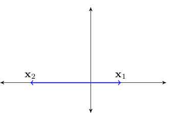
Fig. 57 The vectors \({\bf x}_1\) and \({\bf x}_2\)#
Proof
\(\mathrm{span} \{{\bf x}_1\} \subset \mathrm{span}\{{\bf x}_1, {\bf x}_2\}\) is clear (why?)
To see the reverse, pick any \({\bf y} \in \mathrm{span} \{{\bf x}_1, {\bf x}_2\}\)
By definition,
The right hand side is clearly in \(\mathrm{span} \{{\bf x}_1\}\)
Hence \(\mathrm{span} \{{\bf x}_1, {\bf x}_2\} \subset \mathrm{span} \{{\bf x}_1\}\) as claimed
Implications of Independence#
Let \(X := \{{\bf x}_1,\ldots, {\bf x}_K\} \subset \mathbb{R}^N\)
Fact
If \(X\) is linearly independent, then \(X\) does not contain \({\bf 0}\)
Exercise: Prove it
Fact
If \(X\) is linearly independent, then every subset of \(X\) is linearly independent
Proof
Sketch of proof: Suppose for example that \(\{{\bf x}_1,\ldots, {\bf x}_{K-1}\} \subset X\) is linearly dependent
Then \(\exists \; \alpha_1, \ldots, \alpha_{K-1}\) not all zero with \(\sum_{k=1}^{K-1} \alpha_k {\bf x}_k = {\bf 0}\)
Setting \(\alpha_K =0\) we can write this as \(\sum_{k=1}^K \alpha_k {\bf x}_k = {\bf 0}\)
Not all scalars zero so contradicts linear independence of \(X\)
Fact
If \(X:= \{{\bf x}_1,\ldots, {\bf x}_K\} \subset \mathbb{R}^N\) is linearly independent and \({\bf z}\) is an \(N\)-vector not in \(\mathrm{span}(X)\), then \(X \cup \{ {\bf z} \}\) is linearly independent
Proof
Suppose to the contrary that \(X \cup \{ {\bf z} \}\) is linearly dependent:
If \(\beta=0\), then by (3) we have \(\sum_{k=1}^K \alpha_k {\bf x}_k = {\bf 0}\) and \(\alpha_k \ne 0\) for some \(k\), a contradiction
If \(\beta \ne0\), then by (3) we have
Hence \({\bf z} \in \mathrm{span}(X)\) — contradiction
Unique Representations#
Let
\(X := \{{\bf x}_1,\ldots,{\bf x}_K\} \subset \mathbb{R}^N\)
\({\bf y} \in \mathbb{R}^N\)
We know that if \({\bf y} \in \mathrm{span}(X)\), then exists representation
But when is this representation unique?
Answer: When \(X\) is linearly independent
Fact
If \(X = \{{\bf x}_1,\ldots, {\bf x}_K\} \subset \mathbb{R}^N\) is linearly independent and \({\bf y} \in \mathbb{R}^N\), then there is at most one set of scalars \(\alpha_1,\ldots,\alpha_K\) such that \({\bf y} = \sum_{k=1}^K \alpha_k {\bf x}_k\)
Proof
Suppose there are two such sets of scalars
That is,
Span and Independence#
Here’s one of the most fundamental results in linear algebra
Exchange Lemma
Let \(S\) be a linear subspace of \(\mathbb{R}^N\), and be spanned by \(K\) vectors.
Then any linearly independent subset of \(S\) has at most \(K\)
vectors
Proof: Omitted
Example
If \(X := \{{\bf x}_1, {\bf x}_2, {\bf x}_3\} \subset \mathbb{R}^2\), then \(X\) is linearly dependent
because \(\mathbb{R}^2\) is spanned by the two vectors \({\bf e}_1, {\bf e}_2\)
Fig. 58 Must be linearly dependent#
Example
Recall the plane (flat plane in \(\mathbb{R}^3\) where height coordinate \(x_3\) is zero)
We showed before that \(\mathrm{span}\{{\bf e}_1, {\bf e}_2\} = P\) for
Therefore any three vectors lying in \(P\) are linearly dependent
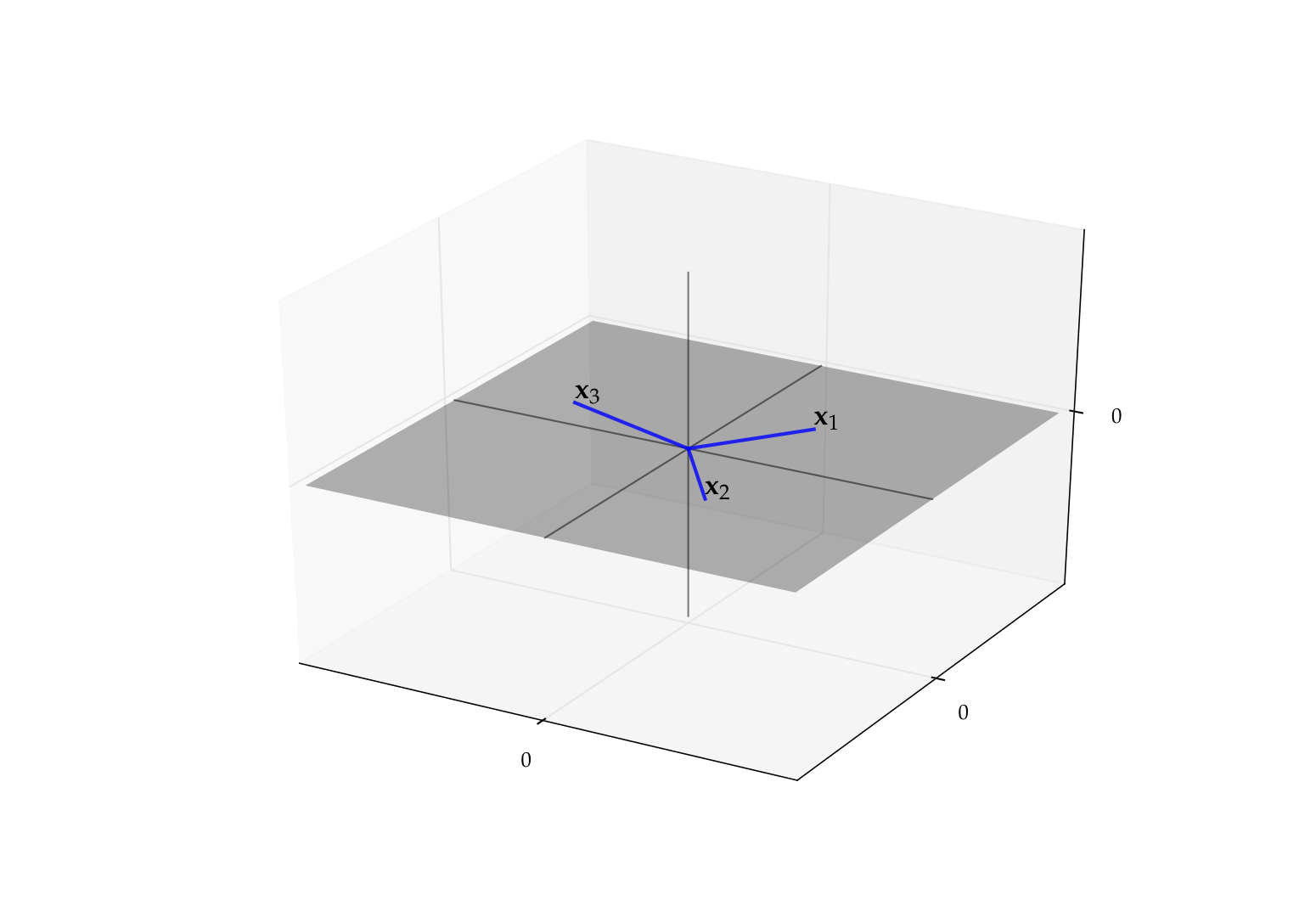
Fig. 59 Any three vectors in \(P\) are linearly dependent#
When Do \(N\) Vectors Span \(\mathbb{R}^N\)?#
In general, linearly independent vectors have a relatively “large” span
No vector is redundant, so each contributes to the span
This helps explain the following fact:
Fact
Let \(X := \{ {\bf x}_1, \ldots, {\bf x}_N \}\) be any \(N\) vectors in \(\mathbb{R}^N\)
\(\mathrm{span}(X) = \mathbb{R}^N\) if and only if \(X\) is linearly independent
Example
The vectors \({\bf x} = (1, 2)\) and \({\bf y} = (-5, 3)\) span \(\mathbb{R}^2\)
Proof
Let prove that
\(X= \{ {\bf x}_1, \ldots, {\bf x}_N \}\) linearly independent \(\implies\) \(\mathrm{span}(X) = \mathbb{R}^N\)
Seeking a contradiction, suppose that
\(X \) is linearly independent
and yet \(\exists \, {\bf z} \in \mathbb{R}^N\) with \({\bf z} \notin \mathrm{span}(X)\)
But then \(X \cup \{{\bf z}\} \subset \mathbb{R}^N\) is linearly independent (why?)
This set has \(N+1\) elements
And yet \(\mathbb{R}^N\) is spanned by the \(N\) canonical basis vectors
Contradiction (of what?)
Next let’s show the converse
\(\mathrm{span}(X) = \mathbb{R}^N\) \(\implies\) \(X= \{ {\bf x}_1, \ldots, {\bf x}_N \}\) linearly independent
Seeking a contradiction, suppose that
\(\mathrm{span}(X) = \mathbb{R}^N\)
and yet \(X\) is linearly dependent
Since \(X\) not independent, \(\exists X_0 \subsetneq X\) with \(\mathrm{span}(X_0) = \mathrm{span}(X)\)
But by 1 this implies that \(\mathbb{R}^N\) is spanned by \(K < N\) vectors
But then the \(N\) canonical basis vectors must be linearly dependent
Contradiction
Bases#
Definition
Let \(S\) be a linear subspace of \(\mathbb{R}^N\)
A set of vectors \(B := \{{\bf b}_1, \ldots, {\bf b}_K\} \subset S\) is called a basis of \(S\) if
\(B\) is linearly independent
\(\mathrm{span}(B) = S\)
Example
Canonical basis vectors form a basis of \(\mathbb{R}^N\)
Indeed, if \(E := \{{\bf e}_1, \ldots, {\bf e}_N\} \subset \mathbb{R}^N\), then
\(E\) is linearly independent – we showed this earlier
\(\mathrm{span}(E) = \mathbb{R}^N\) – we showed this earlier
Example
Recall the plane
We showed before that \(\mathrm{span}\{{\bf e}_1, {\bf e}_2\} = P\) for
Moreover, \(\{{\bf e}_1, {\bf e}_2\}\) is linearly independent (why?)
Hence \(\{{\bf e}_1, {\bf e}_2\}\) is a basis for \(P\)
Fig. 60 The pair \(\{{\bf e}_1, {\bf e}_2\}\) form a basis for \(P\)#
What are the implications of \(B\) being a basis of \(S\)?
In short, every element of \(S\) can be represented uniquely from the smaller set \(B\)
In more detail:
\(B\) spans \(S\) and, by linear independence, every element is needed to span \(S\) — a “minimal” spanning set
Since \(B\) spans \(S\), every \({\bf y}\) in \(S\) can be represented as a linear combination of the basis vectors
By independence, this representation is unique
It’s obvious given the definition that
Fact
If \(B \subset \mathbb{R}^N\) is linearly independent, then \(B\) is a basis of \(\mathrm{span}(B)\)
Example
Let \(B := \{{\bf x}_1, {\bf x}_2\}\) where
We saw earlier that
\(S := \mathrm{span}(B)\) is the plane in \(\mathbb{R}^3\) passing through \({\bf x}_1\), \({\bf x}_2\) and \({\bf 0}\)
\(B\) is linearly independent in \(\mathbb{R}^3\) (dropping either reduces span)
Hence \(B\) is a basis for the plane \(S\)
Fig. 61 The pair \(\{{\bf x}_1, {\bf x}_2\}\) is a basis of its span#
Fundamental Properties of Bases#
Fact
If \(S\) is a linear subspace of \(\mathbb{R}^N\) distinct from \(\{{\bf 0}\}\), then
\(S\) has at least one basis, and
every basis of \(S\) has the same number of elements
Proof
Proof of part 2: Let \(B_i\) be a basis of \(S\) with \(K_i\) elements, \(i=1, 2\)
By definition, \(B_2\) is a linearly independent subset of \(S\)
Moreover, \(S\) is spanned by the set \(B_1\), which has \(K_1\) elements
Hence \(K_2 \leq K_1\)
Reversing the roles of \(B_1\) and \(B_2\) gives \(K_1 \leq K_2\)
Dimension#
Definition
Let \(S\) be a linear subspace of \(\mathbb{R}^N\)
We now know that every basis of \(S\) has the same number of elements
This common number is called the dimension of \(S\)
Example
\(\mathbb{R}^N\) is \(N\) dimensional because the \(N\) canonical basis vectors form a basis
Example
\(P := \{ (x_1, x_2, 0) \in \mathbb{R}^3 \colon x_1, x_2 \in \mathbb{R \}}\) is two dimensional because the first two canonical basis vectors of \(\mathbb{R}^3\) form a basis
Example
In \(\mathbb{R}^3\), a line through the origin is one-dimensional, while a plane through the origin is two-dimensional
Dimension of Spans#
Fact
Let \(X := \{{\bf x}_1,\ldots,{\bf x}_K\} \subset \mathbb{R}^N\)
The following statements are true:
\(\mathrm{dim}(\mathrm{span}(X)) \leq K\)
\(\mathrm{dim}(\mathrm{span}(X)) = K\) \(\;\iff\;\) \(X\) is linearly independent
Proof
Proof that \(\mathrm{dim}(\mathrm{span}(X)) \leq K\)
If not then \(\mathrm{span}(X)\) has a basis with \(M > K\) elements
Hence \(\mathrm{span}(X)\) contains \(M > K\) linearly independent vectors
This is impossible, given that \(\mathrm{span}(X)\) is spanned by \(K\) vectors
Now consider the second claim:
\(X\) is linearly independent \(\implies\) \(\dim(\mathrm{span}(X)) = K\)
Proof: True because the vectors \({\bf x}_1,\ldots,{\bf x}_K\) form a basis of \(\mathrm{span}(X)\)
\(\mathrm{dim}(\mathrm{span}(X)) = K\) \(\implies\) \(X\) linearly independent
Proof: If not then \(\exists \, X_0 \subsetneq X\) such that \(\mathrm{span}(X_0) = \mathrm{span}(X)\)
By this equality and part 1 of the theorem,
Contradiction
Fact
If \(S\) a linear subspace of \(\mathbb{R}^N\), then
Useful implications
The only \(N\)-dimensional subspace of \(\mathbb{R}^N\) is \(\mathbb{R}^N\)
To show \(S = \mathbb{R}^N\) just need to show that \(\dim(S) = N\)
Proof: omitted
Linear Maps#
In this section we investigate one of the most important classes of functions: so-called linear functions
Linear functions play a fundamental role in all fields of science
Linear functions are in one-to-one correspondence with matrices
Even nonlinear functions can often be rewritten as partially linear
The properties of linear functions are closely tied to notions such as
linear combinations, span
linear independence, bases, etc.
Definition
A function \(T \colon \mathbb{R}^K \to \mathbb{R}^N\) is called linear if
Notation:
Linear functions often written with upper case letters
Typically omit parenthesis around arguments when convenient
Example
\(T \colon \mathbb{R} \to \mathbb{R}\) defined by \(Tx = 2x\) is linear
Proof
Take any \(\alpha, \beta, x, y\) in \(\mathbb{R}\) and observe that
Example
The function \(f \colon \mathbb{R} \to \mathbb{R}\) defined by \(f(x) = x^2\) is nonlinear
Proof
Set \(\alpha = \beta = x = y = 1\)
Then
\(f(\alpha x + \beta y) = f(2) = 4\)
But \(\alpha f(x) + \beta f(y) = 1 + 1 = 2\)
Example
Given constants \(c_1\) and \(c_2\), the function \(T \colon \mathbb{R}^2 \to \mathbb{R}\) defined by
is linear
Proof
If we take any \(\alpha, \beta\) in \(\mathbb{R}\) and \({\bf x}, {\bf y}\) in \(\mathbb{R}^2\), then
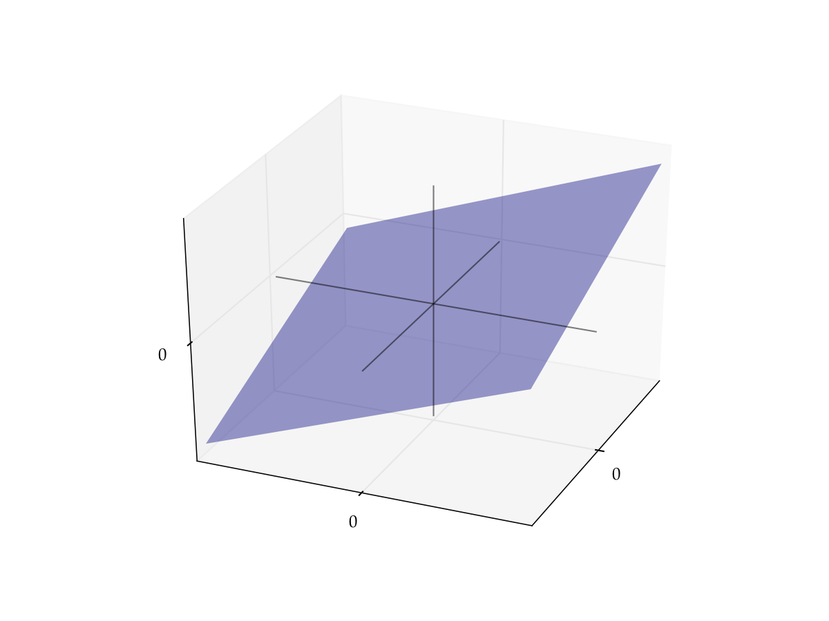
Fig. 62 The graph of \(T {\bf x} = c_1 x_1 + c_2 x_2\) is a plane through the origin#
Remark: Thinking of linear functions as those whose graph is a straight line is not correct
Example
Function \(f \colon \mathbb{R} \to \mathbb{R}\) defined by \(f(x) = 1 + 2x\) is nonlinear
Proof
Take \(\alpha = \beta = x = y = 1\)
Then
\(f(\alpha x + \beta y) = f(2) = 5\)
But \(\alpha f(x) + \beta f(y) = 3 + 3 = 6\)
This kind of function is called an affine function
Let \({\bf a}_1, \ldots, {\bf a}_K\) be vectors in \(\mathbb{R}^N\)
Let \(T \colon \mathbb{R}^K \to \mathbb{R}^N\) be defined by
Exercise: Show that this function is linear
Remarks
This is a generalization of the previous linear examples
In a sense it is the most general representation of a linear map from \(\mathbb{R}^K\) to \(\mathbb{R}^N\)
It is also “the same” as the \(N \times K\) matrix with columns \({\bf a}_1, \ldots, {\bf a}_K\) — more on this later
Implications of Linearity#
Fact
If \(T \colon \mathbb{R}^K \to \mathbb{R}^N\) is a linear map and \({\bf x}_1,\ldots, {\bf x}_J\) are vectors in \(\mathbb{R}^K\), then for any linear combination we have
Proof
Proof for \(J=3\): Applying the def of linearity twice,
Exercise: Show that if \(T\) is any linear function then \(T{\bf 0} = {\bf 0}\)
Fact
If \(T \colon \mathbb{R}^K \to \mathbb{R}^N\) is a linear map, then
Here \({\bf e}_k\) is the \(k\)-th canonical basis vector in \(\mathbb{R}^K\)
Proof
Any \({\bf x} \in \mathbb{R}^K\) can be expressed as \(\sum_{k=1}^K \alpha_k {\bf e}_k\)
Hence \(\mathrm{rng}(T)\) is the set of all points of the form
as we vary \(\alpha_1, \ldots, \alpha_K\) over all combinations
This coincides with the definition of \(\mathrm{span}(V)\)
Example
Let \(T \colon \mathbb{R}^2 \to \mathbb{R}^2\) be defined by
Then
Exercise: Show that \(V := \{T{\bf e}_1, T{\bf e}_2\}\) is linearly independent
We conclude that the range of \(T\) is all of \(\mathbb{R}^2\) (why?)
Definition
The null space or kernel of linear map \(T \colon \mathbb{R}^K \to \mathbb{R}^N\) is
Exercise: Show that \(\mathrm{kernel}(T)\) is a linear subspace of \(\mathbb{R}^K\)
Fact
\(\mathrm{kernel}(T) = \{{\bf 0}\}\) if and only if \(T\) is one-to-one
Proof
Proof of \(\implies\):
Suppose that \(T{\bf x} = T{\bf y}\) for arbitrary \({\bf x}, {\bf y} \in \mathbb{R}^K\)
Then \({\bf 0} = T{\bf x} - T{\bf y} = T({\bf x} - {\bf y})\)
In other words, \({\bf x} - {\bf y} \in \mathrm{kernel}(T)\)
Hence \(\mathrm{kernel}(T) = \{{\bf 0}\}\) \(\implies\) \({\bf x} = {\bf y}\)
Linearity and Bijections#
Recall that an arbitrary function can be
one-to-one (injections)
onto (surjections)
both (bijections)
neither
For linear functions from \(\mathbb{R}^N\) to \(\mathbb{R}^N\), the first three are all equivalent!
In particular,
Fact
If \(T\) is a linear function from \(\mathbb{R}^N\) to \(\mathbb{R}^N\) then all of the following are equivalent:
\(T\) is a bijection
\(T\) is onto/surjective
\(T\) is one-to-one/injective
\(\mathrm{kernel}(T) = \{ {\bf 0} \}\)
The set of vectors \(V := \{T{\bf e}_1, \ldots, T{\bf e}_N\}\) is linearly independent
Definition
If any one of the above equivalent conditions is true, then \(T\) is called nonsingular
Don’t forget: We are talking about \(\mathbb{R}^N\) to \(\mathbb{R}^N\) here

Fig. 63 The case of \(N=1\), nonsingular and singular#
Proof that \(T\) onto \(\iff\) \(V := \{T{\bf e}_1, \ldots, T{\bf e}_N\}\) is linearly independent
Recall that for any linear map \(T\) we have \(\mathrm{rng}(T) = \mathrm{span}(V)\)
Using this fact and the definitions,
(We saw that \(N\) vectors span \(\mathbb{R}^N\) iff linearly indepenent)
Exercise: rest of proof
Fact
If \(T \colon \mathbb{R}^N \to \mathbb{R}^N\) is nonsingular then so is \(T^{-1}\).
What is the implication here?
If \(T\) is a bijection then so is \(T^{-1}\)
Hence the only real claim is that \(T^{-1}\) is also linear
Exercise: prove this statement
Maps Across Different Dimensions#
Remember that the above results apply to maps from \(\mathbb{R}^N\) to \(\mathbb{R}^N\)
Things change when we look at linear maps across dimensions
The general rules for linear maps are
Maps from lower to higher dimensions cannot be onto
Maps from higher to lower dimensions cannot be one-to-one
In either case they cannot be bijections
Fact
For a linear map \(T\) from \(\mathbb{R}^K \to \mathbb{R}^N\), the following statements are true:
If \(K < N\) then \(T\) is not onto
If \(K > N\) then \(T\) is not one-to-one
Proof
Proof of part 1: Let \(K < N\) and let \(T \colon \mathbb{R}^K \to \mathbb{R}^N\) be linear
Letting \(V := \{T{\bf e}_1, \ldots, T{\bf e}_K\}\), we have
Hence \(T\) is not onto
Proof of part 2: \(K > N\) \(\implies\) \(T\) is not one-to-one
Suppose to the contrary that \(T\) is one-to-one
Let \(\alpha_1, \ldots, \alpha_K\) be a collection of vectors such that
We have shown that \(\{T{\bf e}_1, \ldots, T{\bf e}_K\}\) is linearly independent
But then \(\mathbb{R}^N\) contains a linearly independent set with \(K > N\) vectors — contradiction
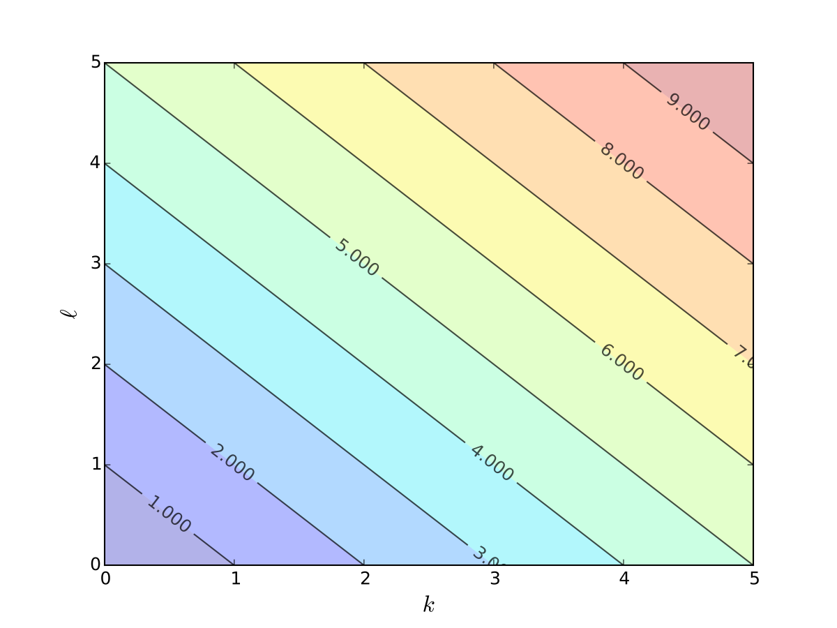
Example
Cost function \(c(k, \ell) = rk + w\ell\) cannot be one-to-one
Matrices and Linear Equations#
As we’ll see, there’s an isomorphic relationship between
matrices
linear maps
Often properties of matrices are best understood via those of linear maps
Typical \(N \times K\) matrix:
Symbol \(a_{ij}\) stands for element in the
\(n\)-th row
\(j\)-th column
Matrices correspond to coefficients of a linear equation
Given the \(a_{ij}\) and \(b_i\), what values of \(x_1, \ldots, x_K\) solve this system?
We now investigate this and other related questions
But first some background on matrices…
An \(N \times K\) matrix also called a
row vector if \(N = 1\)
column vector if \(K = 1\)
Example
Definition
If \(N = K\), then \({\bf A}\) is called square matrix
We use
\(\mathrm{col}_k({\bf A})\) to denote the \(k\)-th column of \({\bf A}\)
\(\mathrm{row}_n({\bf A})\) to denote the \(n\)-th row of \({\bf A}\)
Example
The zero matrix is
The identity matrix is
Algebraic Operations for Matrices#
Addition and scalar multiplication are also defined for matrices
Both are element by element, as in the vector case
Scalar multiplication:
Addition:
Note: that matrices must be same dimension
Multiplication of matrices
Product \({\bf A} {\bf B}\): \(i,j\)-th element is inner product of \(i\)-th row of \({\bf A}\) and \(j\)-th column of \({\bf B}\)
In this display,
Suppose \({\bf A}\) is \(N \times K\) and \({\bf B}\) is \(J \times M\)
\({\bf A} {\bf B}\) defined only if \(K = J\)
Resulting matrix \({\bf A} {\bf B}\) is \(N \times M\)
The rule to remember
Fact
Important: Multiplication is not commutative: it is not in general true that \({\bf A} {\bf B} = {\bf B} {\bf A}\)
In fact \({\bf B} {\bf A}\) is not well-defined unless \(N = M\) also holds
Multiplication of matrix and a vector#
Rules of matrix multiplication#
Fact
Given scalar \(\alpha\) and conformable \({\bf A}\), \({\bf B}\) and \({\bf C}\), we have
\({\bf A} ({\bf B} {\bf C}) = ({\bf A} {\bf B}) {\bf C}\)
\({\bf A} ({\bf B} + {\bf C}) = {\bf A} {\bf B} + {\bf A} {\bf C}\)
\(({\bf A} + {\bf B}) {\bf C} = {\bf A} {\bf C} + {\bf B} {\bf C}\)
\({\bf A} \alpha {\bf B} = \alpha {\bf A} {\bf B}\)
Here ``conformable’’ means operation makes sense
Definition
The \(k\)-th power of a square matrix \({\bf A}\) is
Definition
If it exists, the square root of \({\bf A}\) is written \({\bf A}^{1/2}\) defined as the matrix \({\bf B}\) such that \({\bf B}^2\) is \({\bf A}\)
In matrix multiplication, \({\bf I}\) is the multiplicative unit
That is, assuming conformability, we always have
Exercise: Check it using the definition of matrix multiplication
If \({\bf I}\) is \(K \times K\), then
import numpy as np
A = [[2, 4],
     [4, 2]]
A = np.array(A) # Convert A to array
B = np.identity(2)
print(A,B)
print('Sum:',A+B)
print('Product:',np.dot(A,B))
[[2 4]
 [4 2]] [[1. 0.]
 [0. 1.]]
Sum: [[3. 4.]
 [4. 3.]]
Product: [[2. 4.]
 [4. 2.]]
Matrices as Maps#
Any \(N \times K\) matrix \({\bf A}\) can be thought of as a function \({\bf x} \mapsto {\bf A} {\bf x}\)
In \({\bf A} {\bf x}\) the \({\bf x}\) is understood to be a column vector
It turns out that every such map is linear!
To see this fix \(N \times K\) matrix \({\bf A}\) and let \(T\) be defined by
Pick any \({\bf x}\), \({\bf y}\) in \(\mathbb{R}^K\), and any scalars \(\alpha\) and \(\beta\)
The rules of matrix arithmetic tell us that
So matrices make linear functions
How about examples of linear functions that don’t involve matrices?
There are none!
Fact
If \(T \colon \mathbb{R}^K \to \mathbb{R}^N\) then
Proof
Just above we showed the \(\Longleftarrow\) part
Let’s show the \(\implies\) part
Let \(T \colon \mathbb{R}^K \to \mathbb{R}^N\) be linear
We aim to construct an \(N \times K\) matrix \({\bf A}\) such that
As usual, let \({\bf e}_k\) be the \(k\)-th canonical basis vector in \(\mathbb{R}^K\)
Define a matrix \({\bf A}\) by \(\mathrm{col}_k({\bf A}) = T{\bf e}_k\)
Pick any \({\bf x} = (x_1, \ldots, x_K) \in \mathbb{R}^K\)
By linearity we have
Matrix Product as Composition#
Fact
Let
\({\bf A}\) be \(N \times K\) and \({\bf B}\) be \(K \times M\)
\(T \colon \mathbb{R}^K \to \mathbb{R}^N\) be the linear map \(T{\bf x} = {\bf A}{\bf x}\)
\(U \colon \mathbb{R}^M \to \mathbb{R}^K\) be the linear map \(U{\bf x} = {\bf B}{\bf x}\)
The matrix product \({\bf A} {\bf B}\) corresponds exactly to the composition of \(T\) and \(U\)
Proof
This helps us understand a few things
For example, let
\({\bf A}\) be \(N \times K\) and \({\bf B}\) be \(J \times M\)
\(T \colon \mathbb{R}^K \to \mathbb{R}^N\) be the linear map \(T{\bf x} = {\bf A}{\bf x}\)
\(U \colon \mathbb{R}^M \to \mathbb{R}^J\) be the linear map \(U{\bf x} = {\bf B}{\bf x}\)
Then \({\bf A} {\bf B}\) is only defined when \(K = J\)
This is because \({\bf A} {\bf B}\) corresponds to \(T \circ U\)
But for \(T \circ U\) to be well defined we need \(K = J\)
Then \(U\) maps \(\mathbb{R}^M\) to \(\mathbb{R}^K\) and \(T\) maps \(\mathbb{R}^K\) to \(\mathbb{R}^N\)
Column Space#
Definition
Let \({\bf A}\) be an \(N \times K\) matrix.
The column space of \({\bf A}\) is defined as the span of its columns
Equivalently,
This is exactly the range of the associated linear map
\(T \colon \mathbb{R}^K \to \mathbb{R}^N\) defined by \(T {\bf x} = {\bf A} {\bf x}\)
Example
If
then the span is all linear combinations
These columns are linearly independent (shown earlier)
Hence the column space is all of \(\mathbb{R}^2\) (why?)
Exercise: Show that the column space of any \(N \times K\) matrix is a linear subspace of \(\mathbb{R}^N\)
Rank#
Equivalent questions
How large is the range of the linear map \(T {\bf x} = {\bf A} {\bf x}\)?
How large is the column space of \({\bf A}\)?
The obvious measure of size for a linear subspace is its dimension
Definition
The dimension of \(\mathrm{span}({\bf A})\) is known as the rank of \({\bf A}\)
Because \(\mathrm{span}({\bf A})\) is the span of \(K\) vectors, we have
Definition
\({\bf A}\) is said to have full column rank if
Fact
For any matrix \({\bf A}\), the following statements are equivalent:
\({\bf A}\) is of full column rank
The columns of \({\bf A}\) are linearly independent
If \({\bf A} {\bf x} = {\bf 0}\), then \({\bf x} = {\bf 0}\)
Exercise: Check this, recalling that
import numpy as np
A = [[2.0, 1.0],
     [6.5, 3.0]]
print(f'Rank = {np.linalg.matrix_rank(A)}')
A = [[2.0, 1.0],
     [6.0, 3.0]]
print(f'Rank = {np.linalg.matrix_rank(A)}')
Rank = 2
Rank = 1
\(N \times N\) Linear Equations#
Let’s look at solving linear equations such as \({\bf A} {\bf x} = {\bf b}\)
We start with the “best” case: number of equations \(=\) number of unknowns
Thus,
Take \(N \times N\) matrix \({\bf A}\) and \(N \times 1\) vector \({\bf b}\) as given
Search for an \(N \times 1\) solution \({\bf x}\)
But does such a solution exist? If so is it unique?
The best way to think about this is to consider the corresponding linear map
Equivalent:
\({\bf A} {\bf x} = {\bf b}\) has a unique solution \({\bf x}\) for any given \({\bf b}\)
\(T {\bf x} = {\bf b}\) has a unique solution \({\bf x}\) for any given \({\bf b}\)
\(T\) is a bijection
We already have conditions for linear maps to be bijections
Just need to translate these into the matrix setting
Recall that \(T\) called nonsingular if \(T\) is a linear bijection
Definition
We say that \({\bf A}\) is nonsingular if \(T: {\bf x} \to {\bf A}{\bf x}\) is nonsingular
Equivalent:
\({\bf x} \mapsto {\bf A} {\bf x}\) is a bijection from \(\mathbb{R}^N\) to \(\mathbb{R}^N\)
We now list equivalent conditions for nonsingularity
Fact
Let \({\bf A}\) be an \(N \times N\) matrix
All of the following conditions are equivalent
\({\bf A}\) is nonsingular
The columns of \({\bf A}\) are linearly independent
\(\mathrm{rank}({\bf A}) = N\)
\(\mathrm{span}({\bf A}) = \mathbb{R}^N\)
If \({\bf A} {\bf x} = {\bf A} {\bf y}\), then \({\bf x} = {\bf y}\)
If \({\bf A} {\bf x} = {\bf 0}\), then \({\bf x} = {\bf 0}\)
For each \({\bf b} \in \mathbb{R}^N\), the equation \({\bf A} {\bf x} = {\bf b}\) has a solution
For each \({\bf b} \in \mathbb{R}^N\), the equation \({\bf A} {\bf x} = {\bf b}\) has a unique solution
All equivalent ways of saying that \(T{\bf x} = {\bf A} {\bf x}\) is a bijection!
Example
For condition 5 the equivalence is:
\({\bf A} {\bf x} = {\bf A} {\bf y}\), then \({\bf x} = {\bf y}\)
\(\iff\)
\(T {\bf x} = T {\bf y}\), then \({\bf x} = {\bf y}\)
\(\iff\)
\(T\) is one-to-one
\(\iff\)
Since \(T\) is a linear map from \(\mathbb{R}^N\) to \(\mathbb{R}^N\),
\(T\) is a bijection
Example
For condition 6 the equivalence is:
if \({\bf A} {\bf x} = {\bf 0}\), then \({\bf x} = {\bf 0}\)
\(\iff\)
\(\{{\bf x}: {\bf A}{\bf x} = {\bf 0}\} = \{{\bf 0}\}\)
\(\iff\)
\(\{{\bf x}: T{\bf x} = {\bf 0}\} = \{{\bf 0}\}\)
\(\iff\)
\(\ker{T}=\{{\bf 0}\}\)
\(\iff\)
Since \(T\) is a linear map from \(\mathbb{R}^N\) to \(\mathbb{R}^N\),
\(T\) is a bijection
Example
For condition 7 the equivalence is:
for each \({\bf b}\in\mathbb{R}^N\), the equation \({\bf A}{\bf x} = {\bf b}\) has a solution
\(\iff\)
every \({\bf b}\in\mathbb{R}^N\) has an \({\bf x}\) such that \({\bf A}{\bf x} = {\bf b}\)
\(\iff\)
every \({\bf b}\in\mathbb{R}^N\) has an \({\bf x}\) such that \(T{\bf x} = {\bf b}\)
\(\iff\)
\(T is onto/surjection\)
\(\iff\)
Since \(T\) is a linear map from \(\mathbb{R}^N\) to \(\mathbb{R}^N\),
\(T\) is a bijection
Example
Now consider condition 2: \
The columns of \({\bf A}\) are linearly independent.
Let \({\bf e}_j\) be the \(j\)-th canonical basis vector in \(\mathbb{R}^N\).
Observe that \({\bf A}{\bf e_j} = \mathrm{col}_j({\bf A})\) \(\implies\) \(T{\bf e_j} = \mathrm{col}_j({\bf A})\) \(\implies\) \(V := \{T {\bf e}_1, \ldots, T{\bf e}_N\} =\) columns of \({\bf A}\), and \(V\) is linearly independent if and only if \(T\) is a bijection
Example
Consider a one good linear market system
Treating \(q\) and \(p\) as the unknowns, let’s write in matrix form as
A unique solution exists whenever the columns are linearly independent
so \((b, -d)\) is not a scalar multiple of \({\bf 1}\) \(\iff\) \(b \ne -d\)
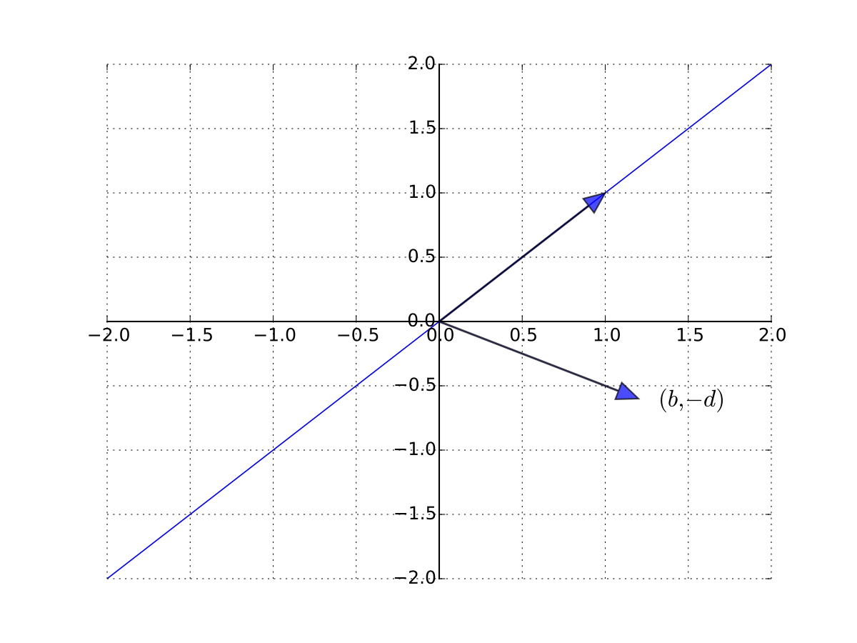
Fig. 64 \((b, -d)\) is not a scalar multiple of \({\bf 1}\)#
Example
Recall in the introduction we try to solve the system \({\bf A} {\bf x} = {\bf b}\) of this form
The problem is that \({\bf A}\) is singular (not nonsingular)
In particular, \(\mathrm{col}_3({\bf A}) = 2 \mathrm{col}_2({\bf A})\)
Inverse Matrices#
Definition
Given square matrix \({\bf A}\), suppose \(\exists\) square matrix \({\bf B}\) such that
Then
\({\bf B}\) is called the inverse of \({\bf A}\), and written \({\bf A}^{-1}\)
\({\bf A}\) is called invertible
Fact
A square matrix \({\bf A}\) is nonsingular if and only if it is invertible
Remark: \({\bf A}^{-1}\) is just the matrix corresponding to the linear map \(T^{-1}\)
Fact
Given nonsingular \(N \times N\) matrix \({\bf A}\) and \({\bf b} \in \mathbb{R}^N\), the unique solution to \({\bf A} {\bf x} = {\bf b}\) is given by
Proof
Since \({\bf A}\) is nonsingular we already know any solution is unique
\(T\) is a bijection, and hence one-to-one
if \({\bf A} {\bf x} = {\bf A} {\bf y} = {\bf b}\) then \({\bf x} = {\bf y}\)
To show that \({\bf x}_b\) is indeed a solution we need to show that \({\bf A} {\bf x}_b = {\bf b}\)
To see this, observe that
Example
Recall the one good linear market system
Suppose that \(a=5\), \(b=2\), \(c=1\), \(d=1.5\)
The matrix system is \({\bf A} {\bf x} = {\bf b}\) where
Since \(b \ne -d\) we can solve for the unique solution
Easy by hand but let’s try on the computer
import numpy as np
from scipy.linalg import inv
A = [[1, 2],
     [1, -1.5]]
b = [5, 1]
q, p = np.dot(inv(A), b) # A^{-1} b
print(f'q={q:.4f} p={p:.4f}')
q=2.7143 p=1.1429
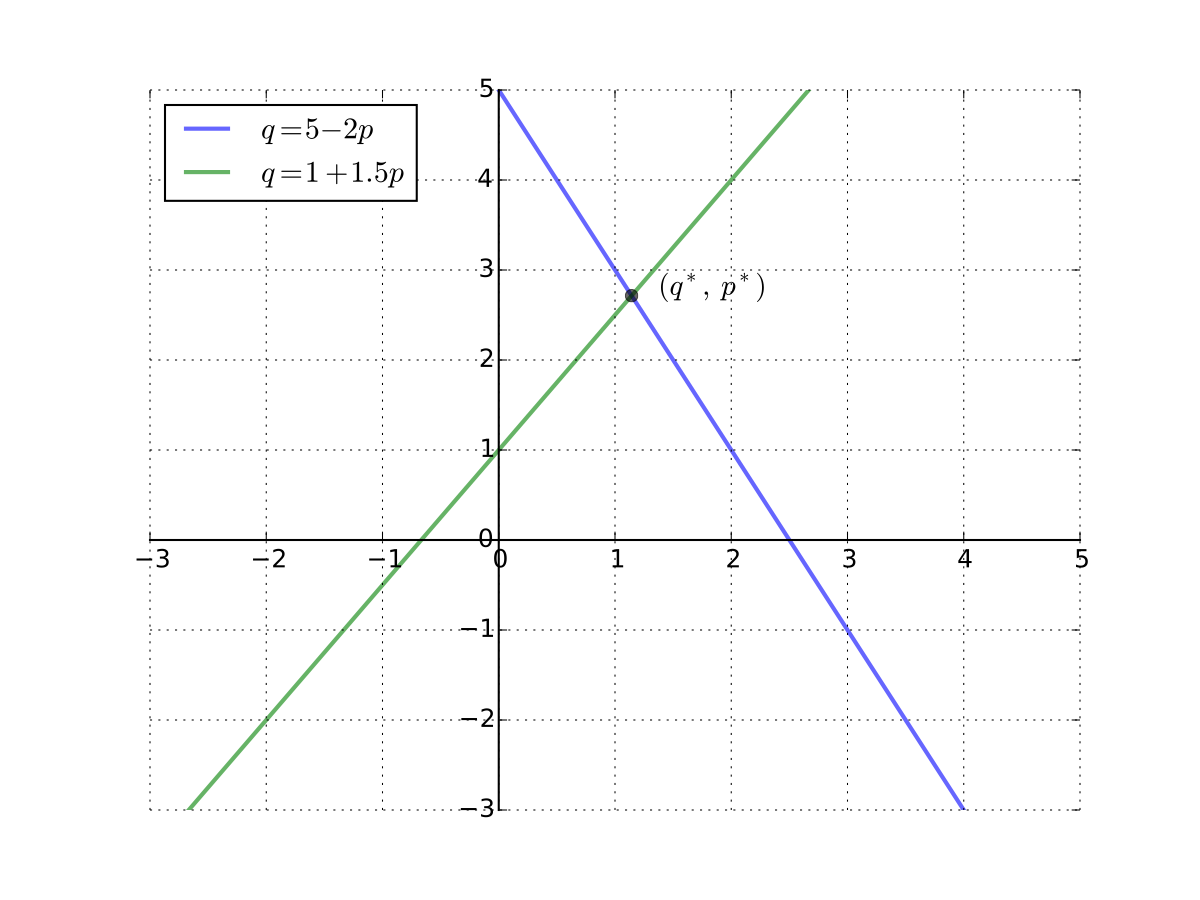
Fig. 65 Equilibrium \((p^*, q^*)\) in the one good case#
Fact
In the \(2 \times 2\) case, the inverse has the form
Example
Example
Consider the \(N\) good linear demand system
Task: take quantities \(q_1, \ldots, q_N\) as given and find corresponding prices \(p_1, \ldots, p_N\) — the “inverse demand curves”
We can write (4) as
where vectors are \(N\)-vectors and \({\bf A}\) is \(N \times N\)
If the columns of \({\bf A}\) are linearly independent then a unique solution exists for each fixed \({\bf q}\) and \({\bf b}\), and is given by
Left and Right Inverses#
Definition
Given square matrix \({\bf A}\), a matrix \({\bf B}\) is called
a left inverse of \({\bf A}\) if \({\bf B} {\bf A} = {\bf I}\)
a right inverse of \({\bf A}\) if \({\bf A} {\bf B} = {\bf I}\)
an inverse of \({\bf A}\) if \({\bf A} {\bf B} = {\bf B} {\bf A} = {\bf I}\)
By definition, a matrix that is both an left inverse and a right inverse is an inverse
Fact
If square matrix \({\bf B}\) is either a left or right inverse for \({\bf A}\), then \({\bf A}\) is nonsingular and \({\bf A}^{-1} = {\bf B}\)
In other words, for square matrices, left inverse \(\iff\) right inverse \(\iff\) inverse
Rules for Inverses#
Fact
If \({\bf A}\) is nonsingular and \(\alpha \ne 0\), then
\({\bf A}^{-1}\) is nonsingular and \(({\bf A}^{-1})^{-1} = {\bf A}\)
\(\alpha {\bf A}\) is nonsingular and \((\alpha {\bf A})^{-1} = \alpha^{-1} {\bf A}^{-1}\)
Proof
Proof of part 2:
It suffices to show that \(\alpha^{-1} {\bf A}^{-1}\) is the right inverse of \(\alpha {\bf A}\)
This is true because
Fact
If \({\bf A}\) and \({\bf B}\) are \(N \times N\) and nonsingular then
\({\bf A} {\bf B}\) is also nonsingular
\(({\bf A} {\bf B})^{-1} = {\bf B}^{-1} {\bf A}^{-1}\)
Proof
Proof I: Let \(T\) and \(U\) be the linear maps corresponding to \({\bf A}\) and \({\bf B}\)
Recall that
\(T \circ U\) is the linear map corresponding to \({\bf A} {\bf B}\)
Compositions of linear maps are linear
Compositions of bijections are bijections
Hence \(T \circ U\) is a linear bijection with \((T \circ U)^{-1} = U^{-1} \circ T^{-1}\)
That is, \({\bf A}{\bf B}\) is nonsingular with inverse \({\bf B}^{-1} {\bf A}^{-1}\)
Proof II:
A different proof that \({\bf A} {\bf B}\) is nonsingular with inverse \({\bf B}^{-1} {\bf A}^{-1}\)
Suffices to show that \({\bf B}^{-1} {\bf A}^{-1}\) is the right inverse of \({\bf A} {\bf B}\)
To see this, observe that
Hence \({\bf B}^{-1} {\bf A}^{-1}\) is a right inverse as claimed
When the Conditions Fail (Singular Case)#
Suppose as before we have
an \(N \times N\) matrix \({\bf A}\)
an \(N \times 1\) vector \({\bf b}\)
We seek a solution \({\bf x}\) to the equation \({\bf A} {\bf x} = {\bf b}\)
What if \({\bf A}\) is singular?
Then \(T{\bf x} = {\bf A} {\bf x}\) is not a bijection, and in fact
\(T\) cannot be onto (otherwise it’s a bijection)
\(T\) cannot be one-to-one (otherwise it’s a bijection)
Hence neither existence nor uniqueness is guaranteed
Example
The matrix \({\bf A}\) with columns
is singular (\({\bf a}_3 = - {\bf a}_2\))
Its column space \(\mathrm{span}({\bf A})\) is just a plane in \(\mathbb{R}^2\)
Recall \({\bf b} \in \mathrm{span}({\bf A})\)
\(\iff\) \(\exists \, x_1, \ldots, x_N\) such that \(\sum_{k=1}^N x_k \mathrm{col}_k({\bf A}) = {\bf b}\)
\(\iff\) \(\exists \, {\bf x}\) such that \({\bf A} {\bf x} = {\bf b}\)
Thus if \({\bf b}\) is not in this plane then \({\bf A} {\bf x} = {\bf b}\) has no solution
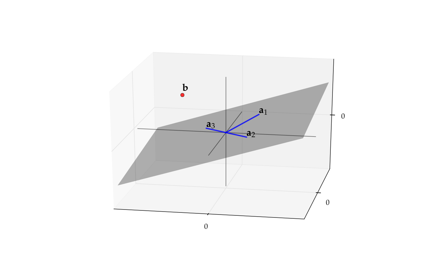
Fig. 66 The vector \({\bf b}\) is not in \(\mathrm{span}({\bf A})\)#
When \({\bf A}\) is \(N \times N\) and singular how rare is scenario \({\bf b} \in \mathrm{span}({\bf A})\)?
Answer: In a sense, very rare
We know that \(\dim(\mathrm{span}({\bf A})) < N\)
Such sets are always “very small” subset of \(\mathbb{R}^N\) in terms of “volume”
A \(K < N\) dimensional subspace has “measure zero” in \(\mathbb{R}^N\)
A “randomly chosen” \({\bf b}\) has zero probability of being in such a set
Example
Consider the case where \(N = 3\) and \(K=2\)
A two-dimensional linear subspace is a 2D plane in \(\mathbb{R}^3\)
This set has no volume because planes have no ``thickness’’
All this means that if \({\bf A}\) is singular then existence of a solution to \({\bf A} {\bf x} = {\bf b}\) typically fails
In fact the problem is worse — uniqueness fails as well
Fact
If \({\bf A}\) is a singular matrix and \({\bf A} {\bf x} = {\bf b}\) has a solution then it has an infinity (in fact a continuum) of solutions
Proof
Let \({\bf A}\) be singular and let \({\bf x}\) be a solution
Since \({\bf A}\) is singular there exists a nonzero \({\bf y}\) with \({\bf A} {\bf y} = {\bf 0}\)
But then \(\alpha {\bf y} + {\bf x}\) is also a solution for any \(\alpha \in \mathbb{R}\) because
Determinants#
Let \(S(N)\) be set of all bijections from \(\{1, \ldots, N\}\) to itself
For \(\pi \in S(N)\) we define the signature of \(\pi\) as
The determinant of \(N \times N\) matrix \({\bf A}\) is then given as
You don’t need to understand or remember this for our course
Fact
In the \(N = 2\) case this definition reduces to
Remark: But you do need to remember this \(2 \times 2\) case
Example
Important facts concerning the determinant
Fact
If \({\bf I}\) is the \(N \times N\) identity, \({\bf A}\) and \({\bf B}\) are \(N \times N\) matrices and \(\alpha \in \mathbb{R}\), then
\(\det({\bf I}) = 1\)
\({\bf A}\) is nonsingular if and only if \(\det({\bf A}) \ne 0\)
\(\det({\bf A}{\bf B}) = \det({\bf A}) \det({\bf B})\)
\(\det(\alpha {\bf A}) = \alpha^N \det({\bf A})\)
\(\det({\bf A}^{-1}) = (\det({\bf A}))^{-1}\)
Example
Thus singularity in the \(2 \times 2\) case is equivalent to
Exercise: Let \({\bf a}_i := \mathrm{col}_i({\bf A})\) and assume that \(a_{ij} \ne 0\) for each \(i, j\)
Show the following are equivalent:
\(a_{11}a_{22} = a_{12} a_{21}\)
\({\bf a}_1 = \lambda {\bf a}_2\) for some \(\lambda \in \mathbb{R}\)
import numpy as np
A = np.random.randn(2, 2) # Random matrix
print(f'A={A}')
print(f'det(A)={np.linalg.det(A)}')
print(f'det(inv(A))={np.linalg.det(np.linalg.inv(A))}')
A=[[ 1.54293968 -1.05347778]
 [ 0.0942124  -0.86642873]]
det(A)=-1.237596590154744
det(inv(A))=-0.808017740154701
As an exercise, let’s now show that any right inverse is an inverse
Fix square \({\bf A}\) and suppose \({\bf B}\) is a right inverse:
Applying the determinant to both sides gives \(\det({\bf A}) \det({\bf B}) = 1\)
Hence \({\bf B}\) is nonsingular (why?) and we can
multiply (5) by \({\bf B}\) to get \({\bf B} {\bf A} {\bf B} = {\bf B}\)
then postmultiply by \({\bf B}^{-1}\) to get \({\bf B} {\bf A} = {\bf I}\)
We see that \({\bf B}\) is also left inverse, and therefore an inverse of \({\bf A}\)
Exercise: Do the left inverse case
\(M \times N\) Linear Systems of Equations#
So far we have considered the nice \(N \times N\) case for equations
number of equations \(=\) number of unknowns
We have to deal with other cases too
Underdetermined systems:
eqs \(<\) unknowns
Overdetermined systems:
eqs \(>\) unknowns
Overdetermined Systems#
Consider the system \({\bf A} {\bf x} = {\bf b}\) where \({\bf A}\) is \(N \times K\) and \(K < N\)
The elements of \({\bf x}\) are the unknowns
More equations than unknowns (\(N > K\))
May not be able to find an \({\bf x}\) that satisfies all \(N\) equations
Let’s look at this in more detail…
Fix \(N \times K\) matrix \({\bf A}\) with \(K < N\)
Let \(T \colon \mathbb{R}^K \to \mathbb{R}^N\) be defined by \(T {\bf x} = {\bf A} {\bf x}\)
We know these to be equivalent:
there exists an \({\bf x} \in \mathbb{R}^K\) with \({\bf A} {\bf x} = {\bf b}\)
\({\bf b}\) has a preimage under \(T\)
\({\bf b}\) is in \(\mathrm{rng}(T)\)
\({\bf b}\) is in \(\mathrm{span}({\bf A})\)
We also know \(T\) cannot be onto (maps small to big space)
Hence \({\bf b} \in \mathrm{span}({\bf A})\) will not always hold
Given our assumption that \(K < N\), how rare is the scenario \({\bf b} \in \mathrm{span}({\bf A})\)?
Answer: We talked about this before — it’s very rare
We know that \(\dim(\mathrm{rng}(T)) = \dim(\mathrm{span}({\bf A})) \leq K < N\)
A \(K < N\) dimensional subspace has “measure zero” in \(\mathbb{R}^N\)
So should we give up on solving \({\bf A} {\bf x} = {\bf b}\) in the overdetermined case?
What’s typically done is we try to find a best approximation
To define ``best’’ we need a way of ranking approximations
The standard way is in terms of Euclidean norm
In particular, we search for the \({\bf x}\) that solves
Details later
Underdetermined Systems#
Now consider \({\bf A} {\bf x} = {\bf b}\) when \({\bf A}\) is \(N \times K\) and \(K > N\)
Let \(T \colon \mathbb{R}^K \to \mathbb{R}^N\) be defined by \(T {\bf x} = {\bf A} {\bf x}\)
Now \(T\) maps from a larger to a smaller place
This tells us that \(T\) is not one-to-one
Hence solutions are not in general unique
In fact the following is true
Exercise: Show that \({\bf A} {\bf x} = {\bf b}\) has a solution and \(K > N\), then the same equation has an infinity of solutions
Remark: Working with underdetermined systems is relatively rare in economics / elsewhere
Transpose#
The transpose of \({\bf A}\) is the matrix \({\bf A}'\) defined by
Example
If
If
Fact
For conformable matrices \({\bf A}\) and \({\bf B}\), transposition satisfies
\(({\bf A}')' = {\bf A}\)
\(({\bf A} {\bf B})' = {\bf B}' {\bf A}'\)
\(({\bf A} + {\bf B})' = {\bf A}' + {\bf B}'\)
\((c {\bf A})' = c {\bf A}'\) for any constant \(c\)
For each square matrix \({\bf A}\),
\(\det({\bf A}') = \det({\bf A})\)
If \({\bf A}\) is nonsingular then so is \({\bf A}'\), and \(({\bf A}')^{-1}= ({\bf A}^{-1})'\)
Definition
A square matrix \({\bf A}\) is called symmetric if \({\bf A}' = {\bf A}\)
Equivalent: \(a_{nk} = a_{kn}\) for all \(n, k\)
Example
Exercise: For any matrix \({\bf A}\), show that \({\bf A}' {\bf A}\) and \({\bf A} {\bf A}'\) are always
well-defined (multiplication makes sense)
symmetric
Definition
The trace of a square matrix is defined by
Fact
\(\mathrm{trace}({\bf A}) = \mathrm{trace}({\bf A}')\)
Fact
If \({\bf A}\) and \({\bf B}\) are square matrices and \(\alpha, \beta \in \mathbb{R}\), then
Fact
When conformable, \(\mathrm{trace}({\bf A} {\bf B}) = \mathrm{trace}({\bf B} {\bf A})\)
Definition
A square matrix \({\bf A}\) is called idempotent if \({\bf A} {\bf A} = {\bf A}\)
Example
The next result is often used in statistics / econometrics:
Fact
If \({\bf A}\) is idempotent, then \(\mathrm{rank}({\bf A}) = \mathrm{trace}({\bf A})\)
Diagonal Matrices#
Consider a square \(N \times N\) matrix \({\bf A}\)
Definition
The \(N\) elements of the form \(a_{nn}\) are called the principal diagonal
A square matrix \({\bf D}\) is called diagonal if all entries off the principal diagonal are zero
Often written as
Incidentally, the same notation works in Python
import numpy as np
D = np.diag((2, 4, 6, 8, 10))
print(D)
[[ 2  0  0  0  0]
 [ 0  4  0  0  0]
 [ 0  0  6  0  0]
 [ 0  0  0  8  0]
 [ 0  0  0  0 10]]
Diagonal systems are very easy to solve
Example
is equivalent to
Fact
If \({\bf C} = \mathrm{diag}(c_1, \ldots, c_N)\) and \({\bf D} = \mathrm{diag}(d_1, \ldots,d_N)\) then
\({\bf C} + {\bf D} = \mathrm{diag}(c_1 + d_1, \ldots, c_N + d_N)\)
\({\bf C} {\bf D} = \mathrm{diag}(c_1 d_1, \ldots, c_N d_N)\)
\({\bf D}^k = \mathrm{diag}(d^k_1, \ldots, d^k_N)\) for any \(k \in \mathbb{N}\)
\(d_n \geq 0\) for all \(n\) \(\implies\) \({\bf D}^{1/2}\) exists and equals
\(d_n \ne 0\) for all \(n\) \(\implies\) \({\bf D}\) is nonsingular and
Proofs: Check 1 and 2 directly, other parts follow
Definition
A square matrix is called lower triangular if every element strictly above the principle diagonal is zero
Example
Definition
A square matrix is called upper triangular if every element strictly below the principle diagonal is zero
Example
Definition
A matrix is called triangular if either upper or lower triangular
Associated linear equations also simple to solve
Example
becomes
Top equation involves only \(x_1\), so can solve for it directly
Plug that value into second equation, solve out for \(x_2\), etc.
Eigenvalues and Eigenvectors#
Let \({\bf A}\) be \(N \times N\)
In general \({\bf A}\) maps \({\bf x}\) to some arbitrary new location \({\bf A} {\bf x}\)
But sometimes \({\bf x}\) will only be scaled:
Definition
If (8) holds and \({\bf x}\) is nonzero, then
\({\bf x}\) is called an eigenvector of \({\bf A}\) and \(\lambda\) is called an eigenvalue
\(({\bf x}, \lambda)\) is called an eigenpair
Clearly \(({\bf x}, \lambda)\) is an eigenpair of \({\bf A}\) \(\implies\) \((\alpha {\bf x}, \lambda)\) is an eigenpair of \({\bf A}\) for any nonzero \(\alpha\)
Example
Let
Then
form an eigenpair because \({\bf x} \ne {\bf 0}\) and
import numpy as np
A = [[1, 2],
     [2, 1]]
eigvals, eigvecs = np.linalg.eig(A)
for i in range(eigvals.size):
  x = eigvecs[:,i]
  lm = eigvals[i]
  print(f'Eigenpair {i}:\n{lm:.5f} --> {x}')
  print(f'Check Ax=lm*x: {np.dot(A, x)} = {lm * x}')
Eigenpair 0:
3.00000 --> [0.70710678 0.70710678]
Check Ax=lm*x: [2.12132034 2.12132034] = [2.12132034 2.12132034]
Eigenpair 1:
-1.00000 --> [-0.70710678  0.70710678]
Check Ax=lm*x: [ 0.70710678 -0.70710678] = [ 0.70710678 -0.70710678]
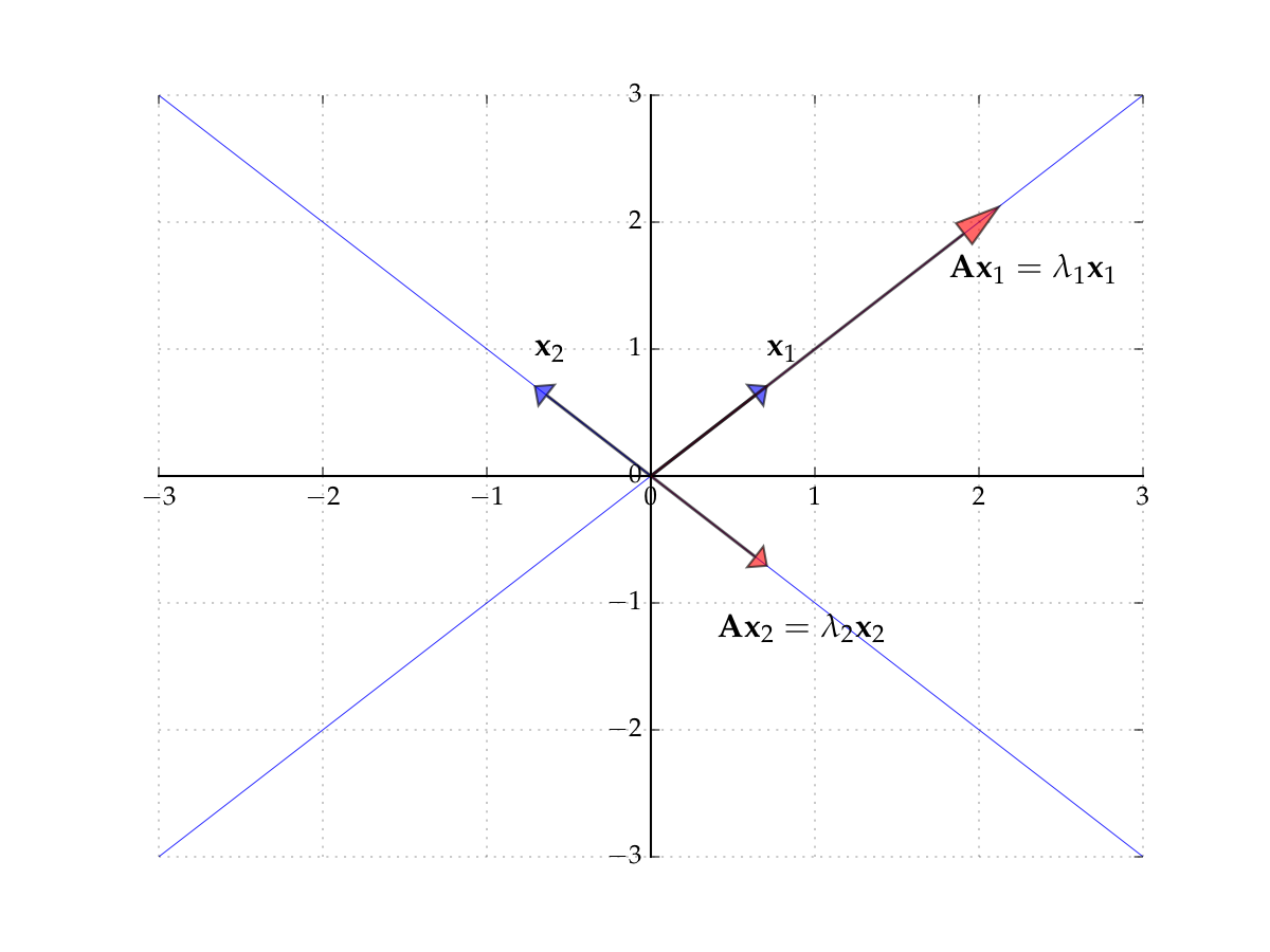
Fig. 67 The eigenvectors of \({\bf A}\)#
Consider the matrix
Induces counter-clockwise rotation on any point by \(90^{\circ}\)
Hint
The rows of the matrix show where the classic basis vectors are translated to.
Hence no point \({\bf x}\) is scaled
Hence there exists no pair \(\lambda \in \mathbb{R}\) and \({\bf x} \ne {\bf 0}\) such that
In other words, no real-valued eigenpairs exist
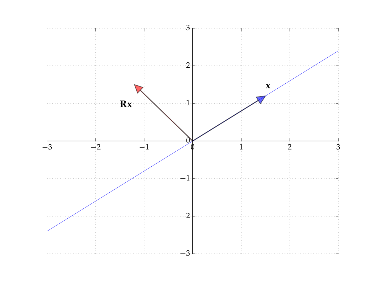
Fig. 68 The matrix \({\bf R}\) rotates points by \(90^{\circ}\)#
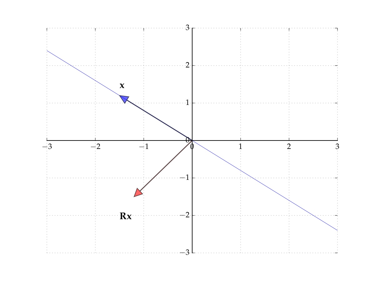
Fig. 69 The matrix \({\bf R}\) rotates points by \(90^{\circ}\)#
But \({\bf R} {\bf x} = \lambda {\bf x}\) can hold if we allow complex values
Example
That is,
Hence \(({\bf x}, \lambda)\) is an eigenpair provided we admit complex values
Note
We do, since this is standard, but will not go into details in this course
Fact
For any square matrix \({\bf A}\)
Proof
Let \({\bf A}\) by \(N \times N\) and let \({\bf I}\) be the \(N \times N\) identity
We have
Example
In the \(2 \times 2\) case,
Hence the eigenvalues of \({\bf A}\) are given by the two roots of
Equivalently,
Diagonalization#
Definition
Square matrix \({\bf A}\) is said to be similar to square matrix \({\bf B}\) if

Fact
If \({\bf A}\) is similar to \({\bf B}\), then \({\bf A}^t\) is similar to \({\bf B}^t\) for all \(t \in \mathbb{N}\)
Proof
Proof for case \(t=2\):
Definition
If \({\bf A}\) is similar to a diagonal matrix, then \({\bf A}\) is called diagonalizable
Fact
Let \({\bf A}\) be diagonalizable with \({\bf A} = {\bf P} {\bf D} {\bf P}^{-1}\) and let
\({\bf D} = \mathrm{diag}(\lambda_1, \ldots, \lambda_N)\)
\({\bf p}_n := \mathrm{col}_n({\bf P})\)
Then \(({\bf p}_n, \lambda_n)\) is an eigenpair of \({\bf A}\) for each \(n\)
Proof
From \({\bf A} = {\bf P} {\bf D} {\bf P}^{-1}\) we get \({\bf A} {\bf P} = {\bf P} {\bf D}\)
Equating \(n\)-th column on each side gives
Moreover \({\bf p}_n \ne {\bf 0}\) because \({\bf P}\) is invertible (which facts?)
Fact
If \(N \times N\) matrix \({\bf A}\) has \(N\) distinct eigenvalues \(\lambda_1, \ldots, \lambda_N\), then \({\bf A}\) is diagonalizable as \({\bf A} = {\bf P} {\bf D} {\bf P}^{-1}\) where
\({\bf D} = \mathrm{diag}(\lambda_1, \ldots, \lambda_N)\)
\(\mathrm{col}_n({\bf P})\) is an eigenvector for \(\lambda_n\)
Example
Let
The eigenvalues of \({\bf A}\) are 2 and 4, while the eigenvectors are
Hence
import numpy as np
from numpy.linalg import inv
A = np.array([[1, -1],
              [3, 5]])
eigvals, eigvecs = np.linalg.eig(A)
D = np.diag(eigvals)
P = eigvecs
print('A =',A,sep='\n')
print('D =',D,sep='\n')
print('P =',P,sep='\n')
print('P^-1 =',inv(P),sep='\n')
print('P*D*P^-1 =',P@D@inv(P),sep='\n')
A =
[[ 1 -1]
 [ 3  5]]
D =
[[2. 0.]
 [0. 4.]]
P =
[[-0.70710678  0.31622777]
 [ 0.70710678 -0.9486833 ]]
P^-1 =
[[-2.12132034 -0.70710678]
 [-1.58113883 -1.58113883]]
P*D*P^-1 =
[[ 1. -1.]
 [ 3.  5.]]
The Euclidean Matrix Norm#
The concept of norm is very helpful for working with vectors: provides notions of distance, similarity, convergence
How about an analogous concept for matrices?
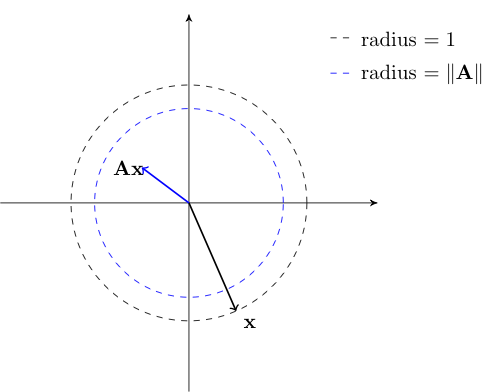
Definition
Given \(N \times K\) matrix \({\bf A}\), denote \(\| {\bf A} \|\) the matrix norm of \({\bf A}\).
Euclidean matrix norm is defined by
In the maximization we can restrict attention to \({\bf x}\) s.t. \(\| {\bf x} \| = 1\)
To see this let
Evidently \(a \geq b\) because max is over a larger domain
To see the reverse let
\({\bf x}_a\) be the maximizer over \({\bf x} \ne {\bf 0}\) and let \(\alpha := 1 / \| {\bf x}_a\|\)
\({\bf x}_b := \alpha {\bf x}_a \)
Then
Definition
If \(\| {\bf A} \| < 1\) then \({\bf A}\) is called contractive — it shrinks the norm
The matrix norm has similar properties to the Euclidean norm
Fact
For conformable matrices \({\bf A}\) and \({\bf B}\), we have
\(\| {\bf A} \| = {\bf 0}\) if and only if all entries of \({\bf A}\) are zero
\(\| \alpha {\bf A} \| = |\alpha| \| {\bf A} \|\) for any scalar \(\alpha\)
\(\| {\bf A} + {\bf B} \| \leq \| {\bf A} \| + \| {\bf B} \|\)
\(\| {\bf A} {\bf B} \| \leq \| {\bf A} \| \| {\bf B} \|\)
The last inequality is called the submultiplicative property of the matrix norm
For square \({\bf A}\) it implies that \(\|{\bf A}^k\| \leq \|{\bf A} \|^k\) for any \(k \in \mathbb{N}\)
Fact
For the diagonal matrix
we have
We can use matrices as elements of sequences
Let \(\{ {\bf A}_j \}\) and \({\bf A}\) be \(N \times K\) matrices
If \(\| {\bf A}_j - {\bf A} \| \to 0\) then we say that \({\bf A}_j\) converges to \({\bf A}\)
If \(\sum_{j=1}^J {\bf A}_j\) converges to some matrix \({\bf B}_{\infty}\) as \(J \to \infty\) we write
In other words,
Neumann Series [optional]#
Consider the difference equation \({\bf x}_{t+1} = {\bf A} {\bf x}_t + {\bf b}\), where
\({\bf x}_t \in \mathbb{R}^N\) represents the values of some variables at time \(t\)
\({\bf A}\) and \({\bf b}\) form the parameters in the law of motion for \({\bf x}_t\)
Question of interest: is there an \({\bf x}\) such that
In other words, we seek an \({\bf x} \in \mathbb{R}^N\) that solves the system of equations
We can get some insight from the scalar case \(x_{t+1} = a x_t + b\)
If \(|a| < 1\), then this equation has the solution
Does an analogous result hold in the vector case \({\bf x} = {\bf A} {\bf x} + {\bf b}\)?
Yes, if we replace condition \(|a| < 1\) with \(\| {\bf A} \| < 1\)
Let \({\bf b}\) be any vector in \(\mathbb{R}^N\) and \({\bf A}\) be an \(N \times N\) matrix
The next result is called the Neumann series lemma
Fact
If \(\| {\bf A}^k \| < 1\) for some \(k \in \mathbb{N}\), then \({\bf I} - {\bf A}\) is invertible and
In this case \({\bf x} = {\bf A} {\bf x} + {\bf b}\) has the unique solution
Proof
Sketch of proof that \(({\bf I} - {\bf A})^{-1} = \sum_{j=0}^{\infty} {\bf A}^j\) for case \(\|{\bf A} \| < 1\)
We have \(({\bf I} - {\bf A}) \sum_{j=0}^{\infty} {\bf A}^j = {\bf I} \) because
How to test the hypotheses of the Neumann series lemma?
Definition
The spectral radius of square matrix \({\bf A}\) is
Here \(|\lambda|\) is the modulus of the possibly complex number \(\lambda\). That is, if \(\lambda = a + ib\), then \(|\lambda| = \sqrt{a^2 + b^2}\).
Quadratic Forms#
Up till now we have studied linear functions extensively
Next level of complexity is quadratic maps
Definition
Let \({\bf A}\) be \(N \times N\) and symmetric, and let \({\bf x}\) be \(N \times 1\)
The quadratic function on \(\mathbb{R}^N\) associated with \({\bf A}\) is the map
The properties of \(Q\) depend on \({\bf A}\)
An \(N \times N\) symmetric matrix \({\bf A}\) is called
nonnegative definite if \({\bf x}' {\bf A} {\bf x} \geq 0\) for all \({\bf x} \in \mathbb{R}^N\)
positive definite if \({\bf x}' {\bf A} {\bf x} > 0\) for all \({\bf x} \in \mathbb{R}^N\) with \({\bf x} \ne {\bf 0}\)
nonpositive definite if \({\bf x}' {\bf A} {\bf x} \leq 0\) for all \({\bf x} \in \mathbb{R}^N\)
negative definite if \({\bf x}' {\bf A} {\bf x} < 0\) for all \({\bf x} \in \mathbb{R}^N\) with \({\bf x} \ne {\bf 0}\)
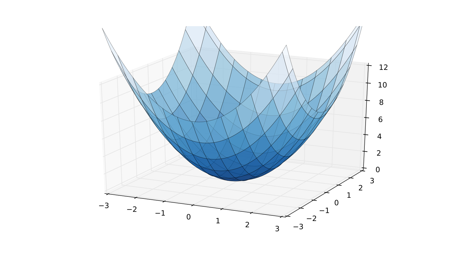
Fig. 70 A positive definite case: \(Q({\bf x}) = {\bf x}' {\bf I} {\bf x}\)#
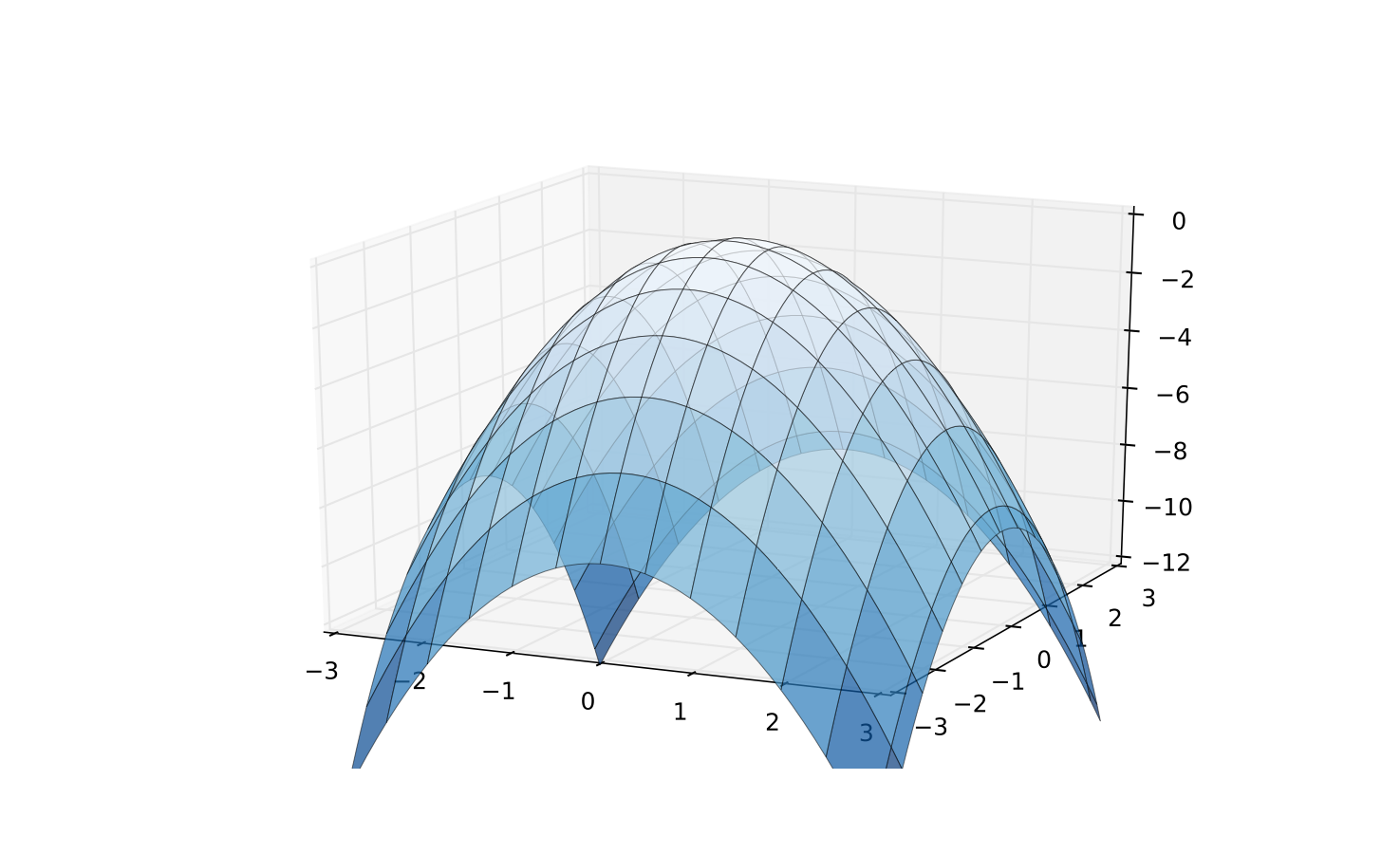
Fig. 71 A negative definite case: \(Q({\bf x}) = {\bf x}'(-{\bf I}){\bf x}\)#
Note that some matrices have none of these properties
\({\bf x}' {\bf A} {\bf x} < 0\) for some \({\bf x}\)
\({\bf x}' {\bf A} {\bf x} > 0\) for other \({\bf x}\)
In this case \({\bf A}\) is called indefinite
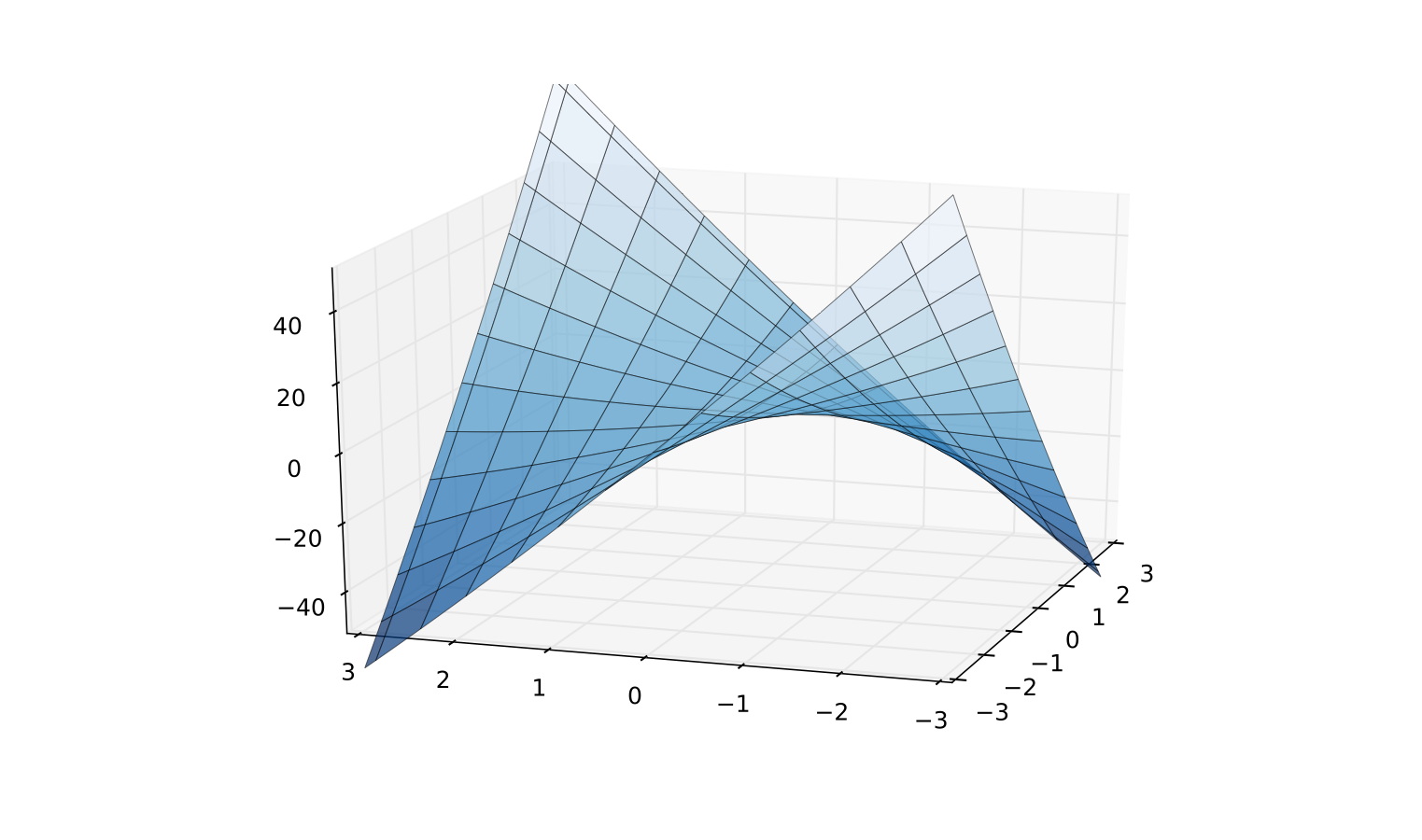
Fig. 72 Indefinite quadratic function \(Q({\bf x}) = x_1^2/2 + 8 x_1 x_2 + x_2^2/2\)#
Fact
A symmetric matrix \({\bf A}\) is
positive definite \(\iff\) all eigenvalues are strictly positive
negative definite \(\iff\) all eigenvalues are strictly negative
nonpositive definite \(\iff\) all eigenvalues are nonpositive
nonnegative definite \(\iff\) all eigenvalues are nonnegative
It follows that
\({\bf A}\) is positive definite \(\implies\) \(\det({\bf A}) > 0\)
In particular, \({\bf A}\) is nonsingular
Extra study material#
Watch excellent video series on linear algebra by Grant Sanderson (3blue1brown) — best visualisations for strong intuition