Exercise set A

General comment on the tutorial exercises

• these questions are not directly assessable and solutions are provided in a separate document

• the aim is to help you better understand the material we have covered so far and start to prepare for actual assessments

• if you are having no particular problems with this course then please carry on to the questions below; if, on the other hand, you are having difficulty with the material, then please read on

• this is an upper level course on mathematics for economists that pushes you beyond the boundaries of the kind of things we do in high school or first year university

• many people find this material hard at first, however, the experience is that anyone who works diligently and consistently can and will do well

Here are few tips on getting through and doing well:

1. It’s hard to “wing” this course, even if you did well at maths in high school. It’s also very hard to follow everything just from the lectures. It takes practice to do well, just like playing guitar or learning a language. The first resource is the lecture slides, and the more often you read them the more the definitions will stick and the material will gel in your head.

2. Each time you are having difficulty with a new concept try googling it. Have a look at Wikipedia, find a video on YouTube, or some of the other online resources. They might phrase or explain the concept in a way that fits better with your brain.

3. Work consistently throughout the semester. Concepts become clearer and more familiar the more times that you go over them—with at least one sleep in between to allow your brain to organize neurons and synapses to store and categorize this new information.

4. Make use of your tutors. They are very knowledgable and are willing to put in time to help anyone who is genuinely trying (although much less inclined to help those who aren’t).

5. Send me feedback if you think it’s something I can help with (e.g., more practice questions on a certain topic) or drop in during my office hours to discuss.

6. Above all, remember that the course material is nontrivial for a reason. Doing straightforward calculations applying well known rules or memorizing “cookbooks” of facts are not particularly useful, mainly because computers are far, far better than humans at these kinds of activities. What is still very useful—probably more than ever—is understanding concepts and how they relate to each other, and building up your ability to digest technical material and think in a logical way. If you complete this course successfully you will have significantly upgraded your mathematical skills.

Finally, here are some tips on doing proofs:

1. In many instances there will be an easy way to do things, if you can spot it. A question that seems to require a long calculation will likely have an easy answer if you know the relevant fact.

2. If you feel stuck, remember that the hardest step is getting started, and for proofs the best place to start is always the relevant definitions. If you are asked to show that the range of a given function is a linear subspace, start by writing down those two definitions. They will tell you more specifically what you need to show. If you’re still stuck, review any facts from the lecture slides related to those definitions. Is there a different way to describe the range of this function? Is there some fact related to linear subspaces that might be helpful?

3. If you’re still stuck, try flipping the problem around. In the previous example, suppose that the range of the function is not a linear subspace. What would that imply? Can you show that such an outcome is impossible?

4. Be patient and don’t rush. You’ll get quicker naturally, with practice.

Question A.1

Let \(f \colon [-1, 1] \to \mathbb{R}\) be defined by \(f(x) = 1 - |x|\), where \(|x|\) is the absolute value of \(x\).

• Is the point \(x = 0\) a maximizer of \(f\) on \([-1, 1]\)?

• Is it a unique maximizer?

• Is it an interior maximizer?

• Is it stationary?

Question A.2

Let \(f \colon \mathbb{R} \to \mathbb{R}\) be defined by \(f(x) = \sin(x)\).

• Write down the set of stationary points of this function.

• Which of these, if any, are maximizers, and which are minimizers?

Tip

When we discussed these kinds of problems it was for functions of the form \(f \colon [a, b] \to \mathbb{R}\). Now the domain is all of \(\mathbb{R}\). However you can apply the same definitions and use similar reasoning. Also, feel free to look up and use any helpful facts on trigonometric functions.

Question A.3: Profit maximization with Cobb-Douglas production and linear costs

A firm uses capital and labor to produce output. When it employs \(k\) units of capital and \(\ell\) units of labor, its output is \(A k^{\alpha} \ell^{\beta}\) units, where \(A\) is a positive number, and \(\alpha + \beta < 1\).

The unit price of capital is \(r\), and the unit price of labor is \(w\); both are non-negative. The firm would like to maximize the profits taking the price \(p\) of the output as given.

The firm’s chief economist Bob presented the following formulation of the firm’s optimization problem to the CEO Alice:

\[ \text{Choose } k, \ell, w \text{ and } r \text{ to maximize } p k^{\alpha} \ell^{\beta} - w \ell - r k \quad \mathrm{s.t.} \quad \alpha + \beta < 1 \]

Questions:

1. Is this formulation of the firm’s optimization problem correct?

• What part reflects the revenue?

• What part reflects the costs?

• What are the choice variables?

• Are there any constraints to be taken into account?

2. Right down the problem after Alice have updated the formulation.

3. Approach the problem as unconstrained maximization, and follow the steps in the lecture to find find all stationary points (solve the FOCs).

4. Write down second order partial derivatives and verify the shape conditions for the profit function.

5. What is the optimal strategy for the firm? Is the maximizer unique? Why?

Question A.4*

Note

Exercises marked with an asterisk (*) are optional and more difficult.

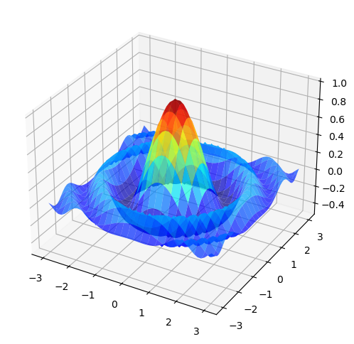
1. Find all stationary points of the function \(f(x, y) = \frac{\cos(x^2 + y^2)}{1 + x^2 + y^2}\).

2. Find all maximizers and minimizers of this function on \(\mathbb{R}^2\).

Hint

Is there a convenient change of variable to convert the problem to a univariate one.

Show code cell content Hide code cell content

from myst_nb import glue
import matplotlib.pyplot as plt
from mpl_toolkits.mplot3d.axes3d import Axes3D
import numpy as np
import scipy as sp
from matplotlib import cm
f = lambda x, y: np.cos(x**2 + y**2) / (1 + x**2 + y**2)
xgrid = np.linspace(-3, 3, 50)
ygrid = xgrid
x, y = np.meshgrid(xgrid, ygrid)
fig = plt.figure(figsize=(8, 6))
ax = fig.add_subplot(111, projection='3d')
ax.plot_surface(x,
                y,
                f(x, y),
                rstride=2, cstride=2,
                cmap=cm.jet,
                alpha=0.7,
                linewidth=0.25)
ax.set_zlim(-0.5, 1.0)
glue("fig_3d", fig, display=False)

g = lambda t: np.cos(t) / (1+t)
gp = lambda t: t * np.sin(t) + np.sin(t) + np.cos(t)
xgrid = np.linspace(0, 10, 200)
fig = plt.figure(figsize=(8, 6))
plt.plot(xgrid, gp(xgrid))
plt.hlines(y=0, xmin=0, xmax=10)
glue("fig_2d", fig, display=False)

res = sp.optimize.root_scalar(gp, bracket=[2, 4], method='brentq')
glue("res_text_1", f"The smallest stationary point is tm={res.root}")
glue("res_text_2", f"The minimum is {g(res.root)}")

'The smallest stationary point is tm=2.889969697678371'

'The minimum is -0.24897613487740497'

Solutions

Question A.1

The point \(x=0\) is indeed a maximizer, since \(f(x) = 1 -|x| \leq 1 = f(0)\) for any \(x \in [-1, 1]\) (\(|x|=0\) if and only if \(x=0\)). It is also a unique maximizer, since no other point is a maximizer (because \(1 -|x| < 1\) for any other \(x\)). It is an interior maximizer since \(0\) is not an end point of \([-1, 1]\). It is not stationary because \(f\) is not differentiable at this point (sketch the graph if you like) and hence cannot satisfy \(f'(x)=0\).

Question A.2

The set \(S\) of stationary points of \(f\) are the points \(x \in \mathbb{R}\) such that \(f'(x) = \cos(x) = 0\). By the definition of the cosine function this is the set

\[ S := \{ x \in \mathbb{R} : x = \pi/2 + k \pi \text{ for } k \in \mathbb{Z} \} \]

Every point in the domain \(\mathbb{R}\) is interior (i.e, not an end point) and the function \(f\) is differentiable, so the set of maximizers will be contained in the set of stationary points. The same is true of the set of minimizers. From the definition of the sine function, we have

\[\begin{split} f(\pi/2 + k \pi) = \begin{cases} 1 & \text{ if $k$ is even} \\ -1 & \text{ if $k$ is odd} \\ \end{cases} \end{split}\]

Hence the set of maximizers is

\[ M^* := \{ x \in \mathbb{R} : x = \pi/2 + k \pi \text{ for } k \text{ an even integer}\} \]

The set of minimizers is

\[ M_* := \{ x \in \mathbb{R} : x = \pi/2 + k \pi \text{ for } k \text{ an odd integer}\} \]

Question A.3

1. The formulation is not correct. The revenue (after reincerting constant \(A\)) is \(p A k^{\alpha} \ell^{\beta}\), the costs are \(w \ell + r k\), and the choice variables are \(k\) and \(\ell\) (\(w\) and \(r\) are not chosen by the firm).
   The constraint \(\alpha + \beta < 1\) is irrelevant for the optimization problem, instead it is a constraint on the parameters for the problem to be well posed. Relevant constraints on the optimization problem are \(k>0\) and \(\ell>0\), they can be first ignored and checked after we solve the unconstrained version of the problem.

2. The correct formulation is (\(A, p, \alpha, \beta, w, r\) are parameters and should be fixed/found out before the firm solves the optimization problem)

\[\begin{split} p A k^{\alpha} \ell^{\beta} - w \ell - r k \rightarrow \max_{k, \ell}\\ \quad \mathrm{s.t.} \quad k \ge 0, \ell \ge 0 \end{split}\]

3. See lecture notes

4. See lecture notes

5. Optimal strategy \(k^*, \ell^*\) are given in the lecture notes. The maximizer is unique because the objective function is strictly concave when \(\alpha+\beta < 1\).

Proof:

We check second order conditions for strict concavity.

What we need: for any \(k, \ell > 0\)

1. \(\pi_{11}(k, \ell) < 0\)

2. \(\pi_{11}(k, \ell) \, \pi_{22}(k, \ell) > \pi_{12}(k, \ell)^2\)

The second order derivatives are

\[\begin{split} \pi_{11}(k,\ell) = (\alpha-1)\alpha pA k^{\alpha-2} \ell^\beta \\ \pi_{22}(k,\ell) = (\beta-1)\beta pA k^{\alpha} \ell^{\beta-2}\\ \pi_{12}(k, \ell) = \alpha \beta pA k^{\alpha-1} \ell^{\beta-1}. \end{split}\]

Since \(\alpha+\beta<1\) and \(\alpha, \beta \geq 0\), we have \(\alpha-1<0\), which implies \(\pi_{11}(k,\ell)<0\) for all \(k, \ell >0\).
Moreover, the second order differentials imply

\[\begin{split} \pi_{11}(k, \ell) \, \pi_{22}(k, \ell) = (\alpha-1)(\beta-1)\alpha \beta p^2 A^2 k^{2\alpha-2} \ell^{2\beta-2}\\ (\pi_{22}(k, \ell))^2 = \alpha^2 \beta^2 p^2 A^2 k^{2\alpha-2} \ell^{2\beta-2}. \end{split}\]

Assuming that all parameters and variables are positive. Then, we obtain \(\pi_{11}(k, \ell) \, \pi_{22}(k, \ell) > \pi_{12}(k, \ell)^2\) if and only if \((\alpha-1)(\beta-1) > \alpha \beta\) if and only if \(1 > \alpha + \beta\).

Question A.4

The graph of \(f(x,y)\) is

Let \(t = x^2+y^2 \geq 0\). The function becomes

\[ f(x,y) = \frac{\cos(x^2+y^2)}{1 + x^2+y^2} = \frac{\cos(t)}{1 + t} =: g(t) \quad (t \geq 0). \]

First note that since \(t \geq 0\) and \(\cos(t) \leq 1\), we have \(g(t)\leq 1\) and \(g(0)=1\). Hence, \(t=0\) is a maximizer for \(g\), or \((x,y)=(0,0)\) is the maximizer for \(f\). It is a unique maximizer, since if \(g(t) < 1\) for \(t >0\).

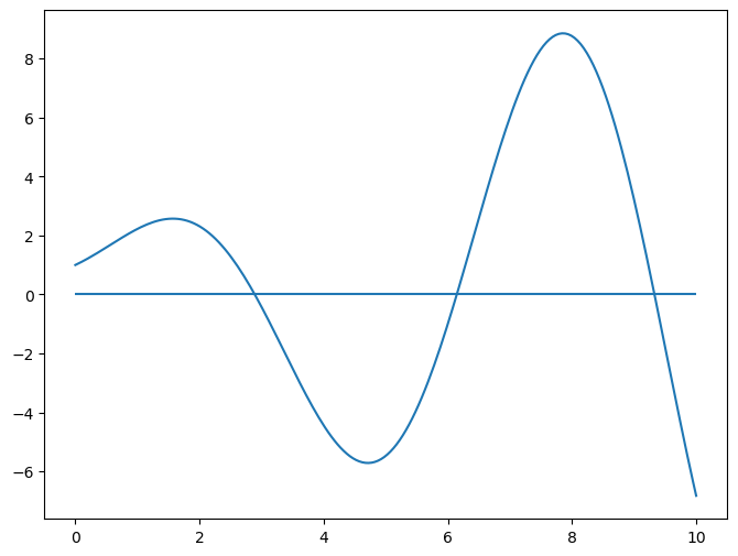
Next, we find the stationary points of \(f\) by finding the stationary points of \(g\). The FOC is

\[ g'(t) = \frac{-\sin(t)(1+t) - \cos(t)}{(1+t)^2} = 0. \]

Since \((1+t)^2>0\), it must be

\[ -\sin(t)(1+t) - \cos(t) = 0 ⇔ t\sin(t) + \sin(t) + \cos(t)=0. \]

The numerical solutions for the smallest stationary point \(t_m\) such that \(\cos(t_m)<0\) are

‘The smallest stationary point is tm=2.889969697678371’

‘The minimum is -0.24897613487740497’

The minimizers are \(\{(x,y)\in\mathbb{R}: x^2+y^2 = t_m\}\). To verify that \(t_m\) is the unique minimizer for \(g\), since \(\cos^2(t) + \sin^2(t)=1\), we rewrite FOC to get

\[\begin{split} t\sin(t) + \sin(t) = \pm \sqrt{1-\sin^2(t)} \\ ⇔ \sin^2(t) = \frac{1}{2 + 2t + t^2} \\ ⇔ \cos^2(t) = 1 - \frac{1}{2+2t + t^2}=\frac{(1+t)^2}{2+2t + t^2}\\ ⇒ g(t) = \frac{\cos(t)}{1+t} = \pm \frac{1}{\sqrt{2+2t +t^2}} \qquad (\text{$t$ is stationary point}). \end{split}\]

Therefore, the smallest stationary point such that \(\cos(t) < 0\) will be the unique minimizer for \(g\).