Basics of real analysis

ECON2125/6012 Lecture 4
Fedor Iskhakov

Announcements & Reminders

1. The first test is due before the next lecture!

• The test will be published tomorrow (before midnight on Friday)

• The test will include multiple choice questions (where multiple options can be correct), True/False questions and open response questions where you may need to upload a file

• Please, find the practice test on Wattle and make sure you are comfortable with the setup, including uploading an image/pdf file

• Tests are timed: practice paying attention to the countdown timer

• The deadline for submission of the first test is midnight on Wednesday, August 23

2. I am traveling next week, no face-to-face lecture on August 24!

• DSE summer school and conference

Plan for this lecture

Continuing with revision of fundamental concepts and ideas

1. Sequences

2. Convergence and limits

3. Differentiation, Taylor series

4. Analysis in ${\mathbb{R}}^n$

5. Open and closed sets

6. Continuity of functions

Mainly review of key ideas

Supplementary reading:

• Simon & Blume: 12.1, 12.2, 12.3, 12.4, 12.5 10.1, 10.2, 10.3, 10.4, 13.4

• Sundaram: 1.1.1, 1.1.2, 1.2.1, 1.2.2, 1.2.3, 1.2.7, 1.2.8, 1.4.1

Analysis in $\mathbb{R}$

Example

Let $F(x)$ be a profit function, so for solving profit maximization we have to solve $f(x)=0$ where $f(x)=F^{\prime }(x)$.

Or: we want to solve an equation $g(x)=y$ for $x$, equivalently $f(x)=g(x)-y$

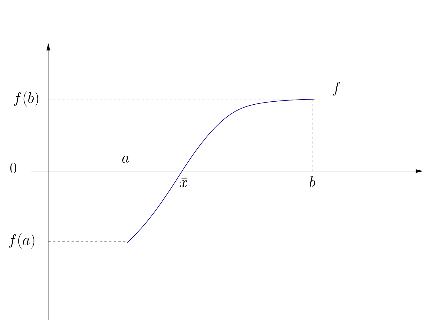
Fig. 31 Existence of a root

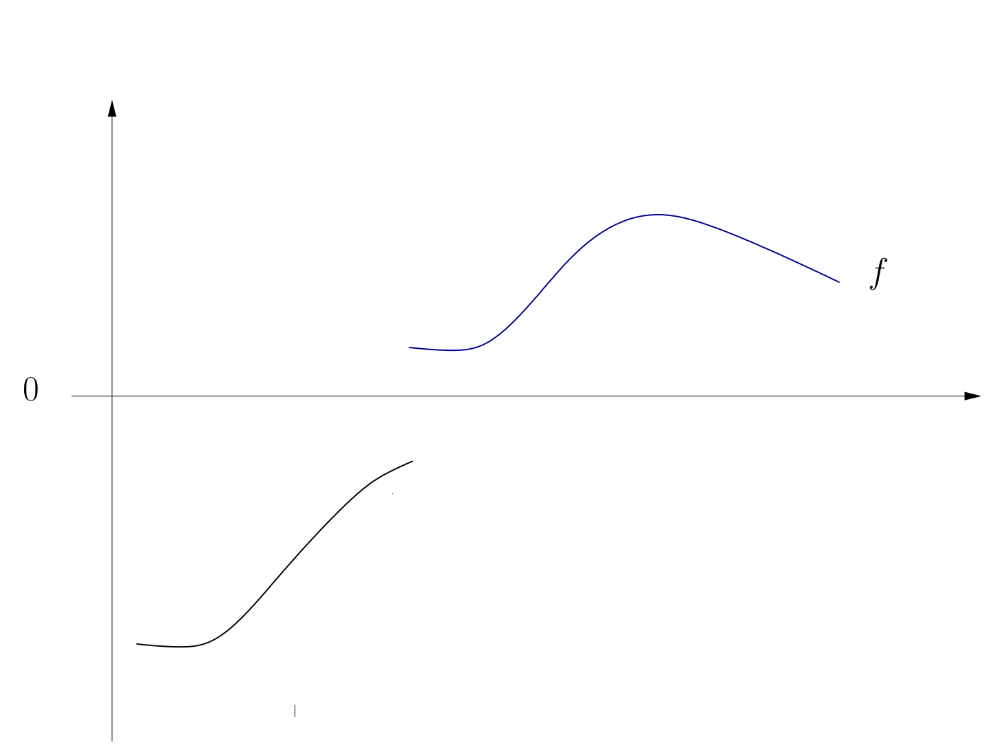
Fig. 32 Non-existence of a root

One answer: a solution exists under certain conditions including continuity.

Questions:

• So how can I tell if $f$ is continuous?

• Can we weaken the continuity assumption?

• Does this work in multiple dimensions?

• When is the root unique?

• How can we compute it?

These are typical problems in analysis

Bounded sets

Definition

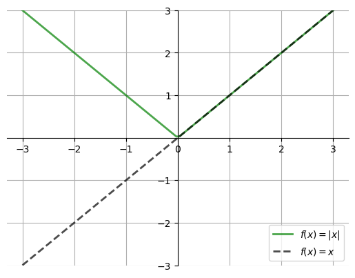
The absolute value of $x\in \mathbb{R}$ denoted $|x|$ is $|x|:=max\{x,-x\}$.

Show code cell source Hide code cell source

import numpy as np
import matplotlib.pyplot as plt

def subplots():
    "Custom subplots with axes throught the origin"
    fig, ax = plt.subplots()

    # Set the axes through the origin
    for spine in ['left', 'bottom']:
        ax.spines[spine].set_position('zero')
    for spine in ['right', 'top']:
        ax.spines[spine].set_color('none')
    
    ax.grid()
    return fig, ax

fig, ax = subplots()

ax.set_ylim(-3, 3)
ax.set_yticks((-3, -2, -1, 1, 2, 3))
x = np.linspace(-3, 3, 100)
ax.plot(x, np.abs(x), 'g-', lw=2, alpha=0.7, label=r'$f(x) = |x|$')
ax.plot(x, x, 'k--', lw=2, alpha=0.7, label=r'$f(x) = x$')
ax.legend(loc='lower right')

plt.show()

Fact

For any $x,y\in \mathbb{R}$, the following statements hold

1. $|x|\le y$ if and only if $-y\le x\le y$

2. $|x|<y$ if and only if $-y<x<y$

3. $|x|=0$ if and only if $x=0$

4. $|xy|=|x||y|$

5. $|x+y|\le |x|+|y|$

Last inequality is called the triangle inequality

Using these rules, let’s show that if $x,y,z\in \mathbb{R}$, then

1. $|x-y|\le |x|+|y|$

2. $|x-y|\le |x-z|+|z-y|$

Proof

Hint: $x-y=x-z+z-y$

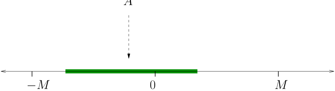
Definition

$A\subset \mathbb{R}$ is called bounded if $\mathrm{\exists }M\in \mathbb{R}$ s.t. $|x|\le M$, all $x\in A$

Example

Every finite subset $A$ of $\mathbb{R}$ is bounded

Set $M:=max\{|a|:a\in A\}$

Example

$\mathbb{N}$ is unbounded

For any $M\in \mathbb{R}$ there is an $n$ that exceeds it

Example

$(a,b)$ is bounded for any $a$ and $b$

Proof

We have to show that each $x\in (a,b)$ satisfies $|x|\le M:=max\{|a|,|b|\}$

$$x\in (a,b)⟺a<x<b$$

Cases:

1. $0\le a\le b⟹x>0,x=|x|<|b|=b=max\{|a|,|b|\}$

2. $a\le b\le 0⟹a<x<0,|x|=-x<-a=|a|=max\{|a|,|b|\}$

3. $a\le 0\le b⟹$

$$\begin{array}{r}\{\begin{array}{l}|x|<|b|,x\ge 0\\ |x|<|a|,x<0\end{array}⟹|x|<max\{|a|,|b|\}\text{ from 1. and 2.}\end{array}$$

Fact

If $A$ and $B$ are bounded sets then so is $A\cup B$

Proof

Let $A$ and $B$ be bounded sets and let $C:=A\cup B$

By definition, $\mathrm{\exists }{M}_A$ and $M_B$ with

$$|a|\le M_A,\text{ all }a\in A,|b|\le M_B,\text{ all }b\in B$$

Let $M_C:=max\{M_A,M_B\}$ and fix any $x\in C$

$$x\in C⟹x\in A\text{ or }x\in B$$

$$\text{therefore }|x|\le M_A\text{or}|x|\le M_B$$

$$\text{therefore }|x|\le M_C$$

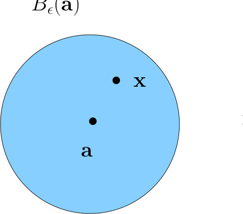
Epsilon-balls ($ϵ$-balls)

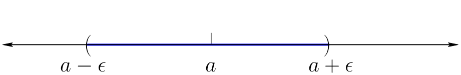
Definition

Given $ϵ>0$ and $a\in \mathbb{R}$, the $ϵ$-ball around $a$ is

$$B_{ϵ}(a):=\{x\in \mathbb{R}:|a-x|<ϵ\}$$

Equivalently,

$$B_{ϵ}(a)=\{x\in \mathbb{R}:a-ϵ<x<a+ϵ\}$$

Exercise: Check equivalence

Fact

If $x$ is in every $ϵ$-ball around $a$ then $x=a$

Proof

Suppose to the contrary that

• $x$ is in every $ϵ$-ball around $a$ and yet $x\ne a$

Since $x$ is not $a$ we must have $|x-a|>0$

Set $ϵ:=|x-a|$

Since $ϵ>0$, we have $x\in B_{ϵ}(a)$

This means that $|x-a|<ϵ$

That is, $|x-a|<|x-a|$

Contradiction!

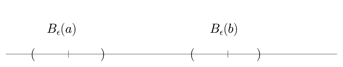
Fact

If $a\ne b$, then $\mathrm{\exists }ϵ>0$ such that $B_{ϵ}(a)$ and $B_{ϵ}(b)$ are disjoint.

Proof

Let $a,b\in \mathbb{R}$ with $a\ne b$

If we set $ϵ:=|a-b|/2$, then $B_{ϵ}(a)$ and $B_{ϵ}(b)$ are disjoint

To see this, suppose to the contrary that $\mathrm{\exists }x\in B_{ϵ}(a)\cap B_{ϵ}(B)$

Then $|x-a|<|a-b|/2$ and $|x-b|<|a-b|/2$

But then

$$|a-b|\le |a-x|+|x-b|<|a-b|/2+|a-b|/2=|a-b|$$

Contradiction!

Sequences

Definition

A sequence is a function from $\mathbb{N}$ to $\mathbb{R}$

To each $n\in \mathbb{N}$ we associate one $x_n\in \mathbb{R}$

Typically written as $\{x_n{\}}_{n=1}^{\mathrm{\infty }}$ or $\{x_n\}$ or $\{x_1,x_2,x_3,\dots \}$

Example

• $\{x_n\}=\{2,4,6,\dots \}$

• $\{x_n\}=\{1,1/2,1/4,\dots \}$

• $\{x_n\}=\{1,-1,1,-1,\dots \}$

• $\{x_n\}=\{0,0,0,\dots \}$

Definition

Sequence $\{x_n\}$ is called

• bounded if $\{x_1,x_2,\dots \}$ is a bounded set

• monotone increasing if $x_{n+1}\ge x_n$ for all $n$

• monotone decreasing if $x_{n+1}\le x_n$ for all $n$

• monotone if it is either monotone increasing or monotone decreasing

Example

• $x_n=1/n$ is monotone decreasing, bounded

• $x_n=(-1{)}^n$ is not monotone but is bounded

• $x_n=2n$ is monotone increasing but not bounded

Convergence

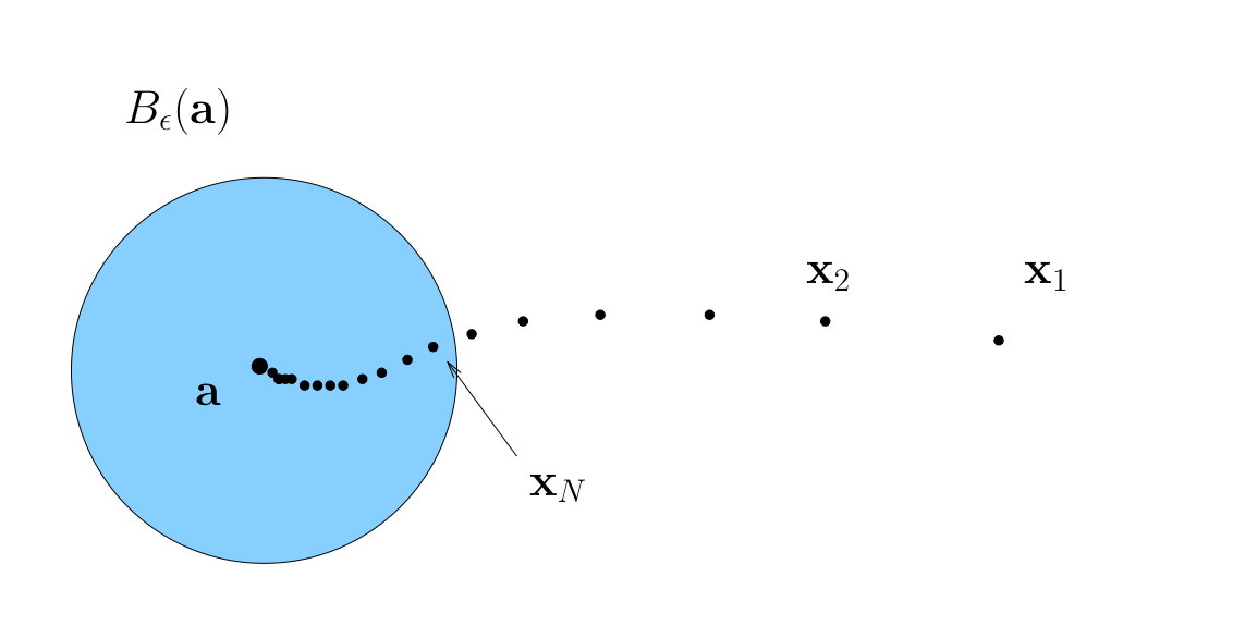
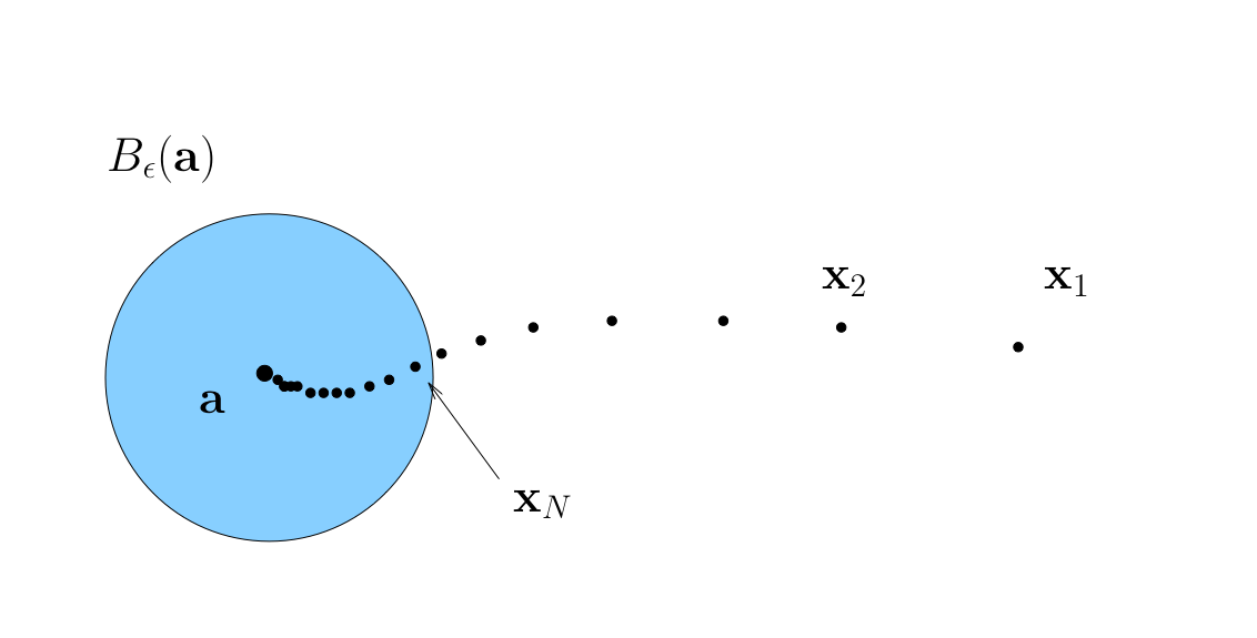
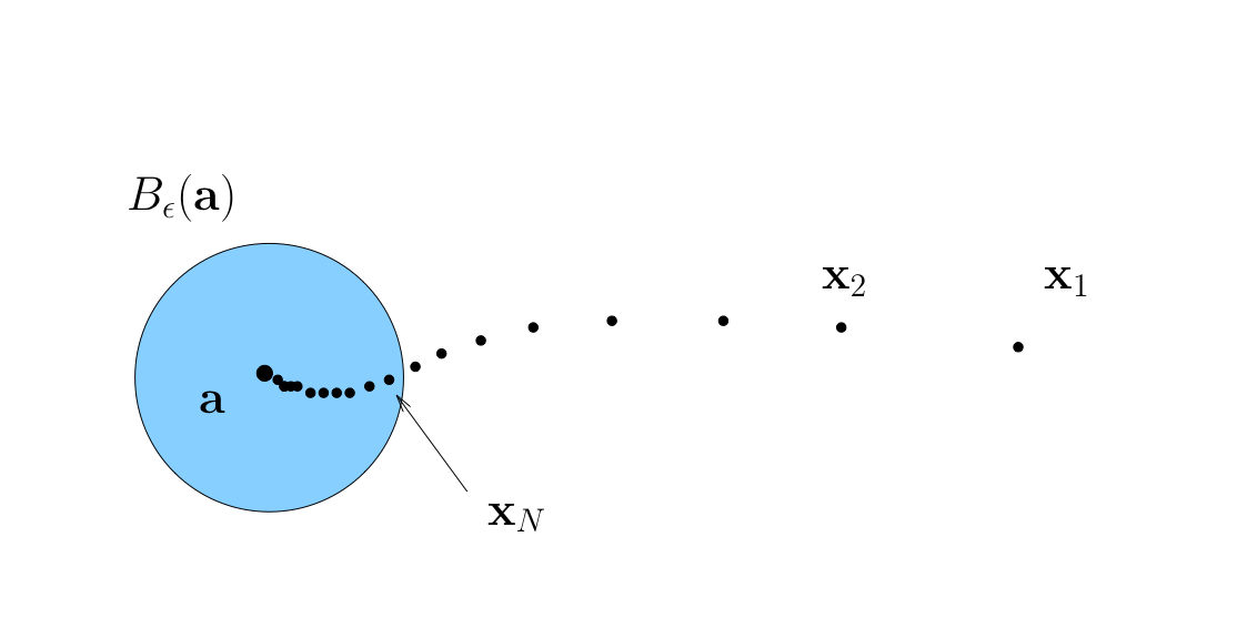
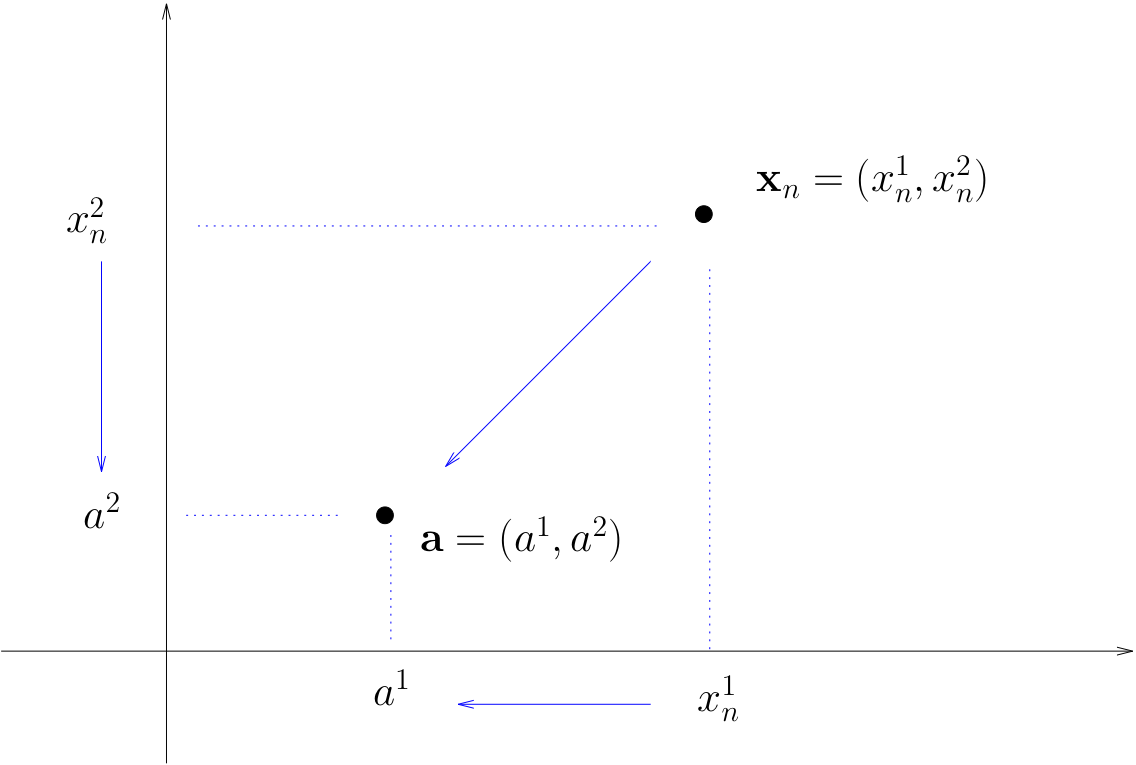
Let $a\in \mathbb{R}$ and let $\{x_n\}$ be a sequence

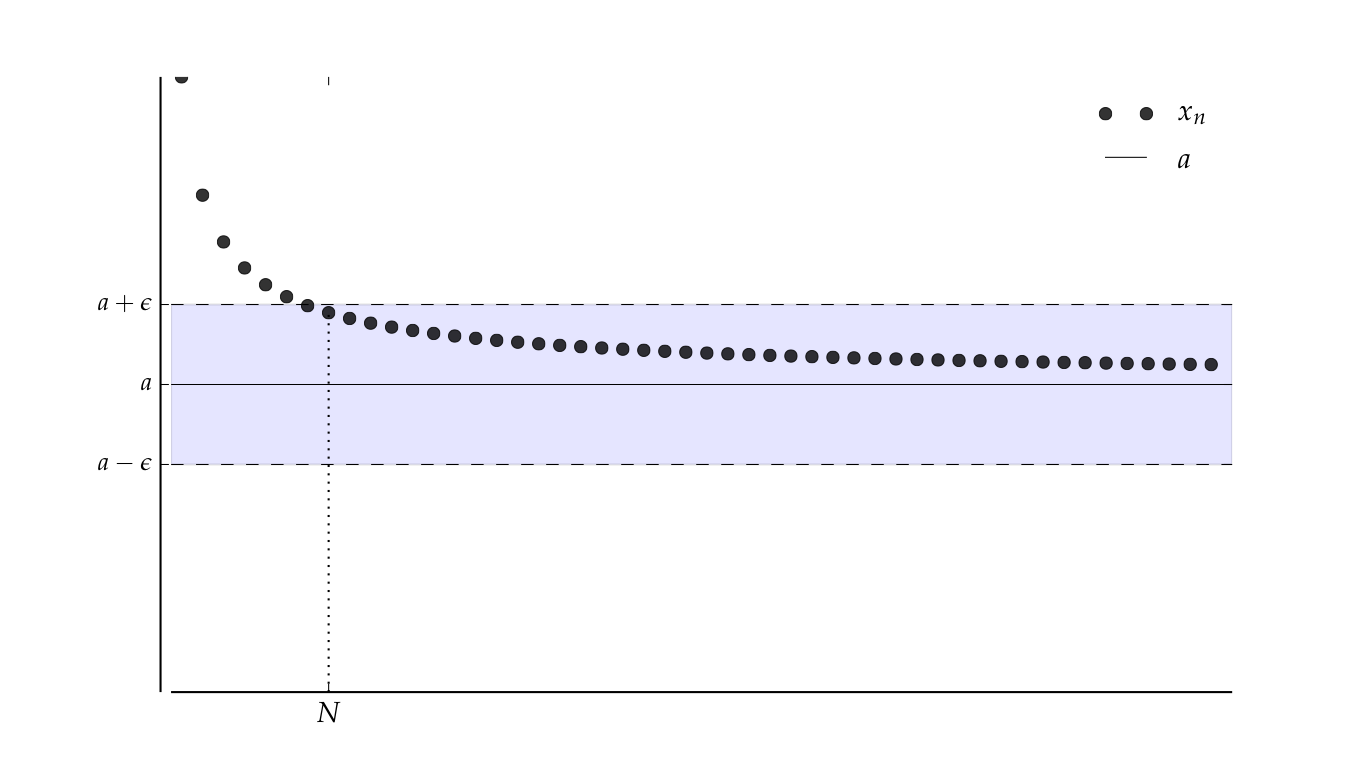
Suppose, for any $ϵ>0$, we can find an $N\in \mathbb{N}$ such that

$$x_n\in B_{ϵ}(a)\text{ for all }n\ge N$$

Then $\{x_n\}$ is said to converge to $a$

Convergence to $a$ in symbols,

$$\mathrm{\forall }ϵ>0,\mathrm{\exists }N\in \mathbb{N}\text{ such that }n\ge N⟹x_n\in B_{ϵ}(a)$$

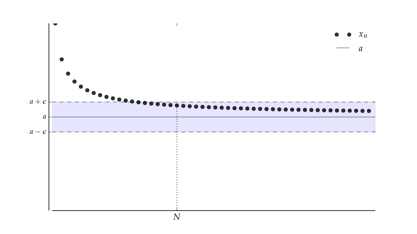
The sequence $\{x_n\}$ is eventually in this $ϵ$-ball around $a$

…and this one

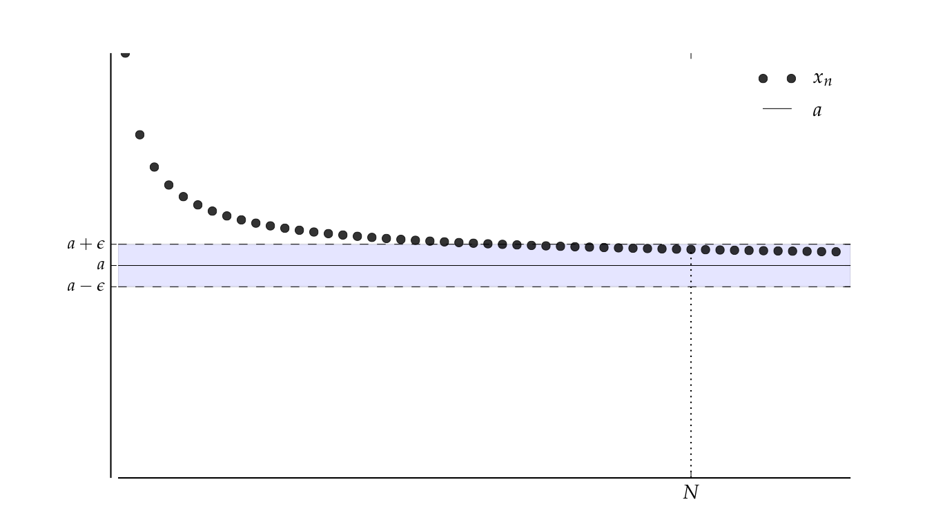
…and this one

…and this one

Definition

The point $a$ is called the limit of the sequence, denoted

$$x_n\to a\text{ as }n\to \mathrm{\infty }\text{ or }\underset{n\to \mathrm{\infty }}{lim}{x}_n=a,$$

if

$$\mathrm{\forall }ϵ>0,\mathrm{\exists }N\in \mathbb{N}\text{ such that }n\ge N⟹x_n\in B_{ϵ}(a)$$

We call $\{x_n\}$ convergent if it converges to some limit in $\mathbb{R}$

Example

$\{x_n\}$ defined by $x_n=1+1/n$ converges to $1$:

$$x_n\to 1\mathrm{as}n\to \mathrm{\infty }$$

$$\underset{n\to \mathrm{\infty }}{lim}{x}_n=1$$

To prove this must show that $\mathrm{\forall }ϵ>0$, there is an $N\in \mathbb{N}$ such that

$$n\ge N⟹|x_n-1|<ϵ$$

To show this formally we need to come up with an “algorithm”

1. You give me any $ϵ>0$

2. I respond with an $N$ such that equation above holds

In general, as $ϵ$ shrinks, $N$ will have to grow

Proof

Here’s how to do this for the case $1+1/n$ converges to $1$

First pick an arbitrary $ϵ>0$

Now we have to come up with an $N$ such that

$$n\ge N⟹|1+1/n-1|<ϵ$$

Let $N$ be the first integer greater than $1/ϵ$

Then

$$n\ge N⟹n>1/ϵ⟹1/n<ϵ⟹|1+1/n-1|<ϵ$$

Remark: Any $N^{\prime }>N$ would also work

Example

The sequence $x_n=2^{-n}$ converges to $0$ as $n\to \mathrm{\infty }$

Proof

Must show that, $\mathrm{\forall }ϵ>0$, $\mathrm{\exists }N\in \mathbb{N}$ such that

$$n\ge N⟹|2^{-n}-0|<ϵ$$

So pick any $ϵ>0$, and observe that

$$|2^{-n}-0|<ϵ⟺2^{-n}<ϵ⟺n>-\frac{\ln ϵ}{\ln 2}$$

Hence we take $N$ to be the first integer greater than $-\ln ϵ/\ln 2$

Then

$$n\ge N⟹n>-\frac{\ln ϵ}{\ln 2}⟹|2^{-n}-0|<ϵ$$

What if we want to show that $x_n\to a$ fails?

To show convergence fails we need to show the negation of

$$\mathrm{\forall }ϵ>0,\mathrm{\exists }N\in \mathbb{N}\mathrm{such}\mathrm{that}n\ge N⟹x_n\in B_{ϵ}(a)$$

Negation: there is an $ϵ>0$ where we can’t find any such $N$

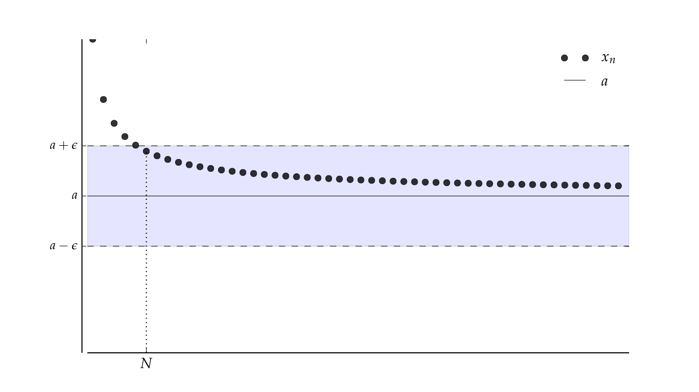
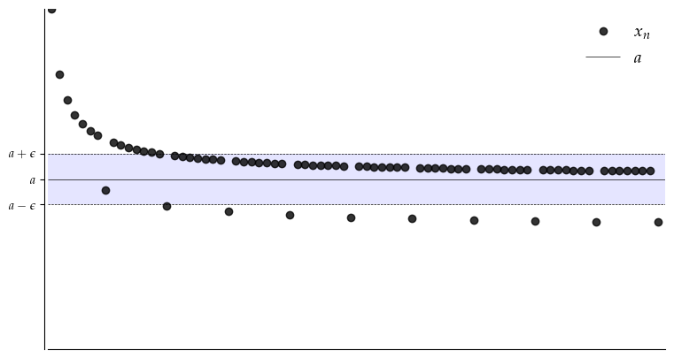
More specifically, $\mathrm{\exists }ϵ>0$ such that, which ever $N\in \mathbb{N}$ we look at, there’s an $n\ge N$ with $x_n$ outside $B_{ϵ}(a)$

One way to say this: there exists a $B_{ϵ}(a)$ such that $x_n\notin B_{ϵ}(a)$ again and again as $n\to \mathrm{\infty }$.

This is the kind of picture we’re thinking of

Show code cell source Hide code cell source

from __future__ import division
import matplotlib.pyplot as plt
import numpy as np

from matplotlib import rc
rc('font',**{'family':'serif','serif':['Palatino']})
rc('text', usetex=True)

N = 80
epsilon = 0.15
a = 1

def x(n):
    return 1 + 1/(n**(0.7)) - 0.3 * (n % 8 == 0)
def subplots(fs):
    "Custom subplots with axes throught the origin"
    fig, ax = plt.subplots(figsize=fs)
    # Set the axes through the origin
    for spine in ['left', 'bottom']:
        ax.spines[spine].set_position('zero')
    for spine in ['right', 'top']:
        ax.spines[spine].set_color('none')
    return fig, ax

fig, ax = subplots((9, 5))  

xmin, xmax = 0.5, N+1
ax.set_xlim(xmin, xmax)
ax.set_ylim(0, 2)

n = np.arange(1, N+1)
ax.set_xticks([])
ax.plot(n, x(n), 'ko', label=r'$x_n$', alpha=0.8)

ax.hlines(a, xmin, xmax, color='k', lw=0.5, label='$a$')
ax.hlines([a - epsilon, a + epsilon], xmin, xmax, color='k', lw=0.5, linestyles='dashed')

ax.fill_between((xmin, xmax), a - epsilon, a + epsilon, facecolor='blue', alpha=0.1)

ax.set_yticks((a - epsilon, a, a + epsilon))
ax.set_yticklabels((r'$a - \epsilon$', r'$a$', r'$a + \epsilon$'))

ax.legend(loc='upper right', frameon=False, fontsize=14)
plt.show()

Example

The sequence $x_n=(-1{)}^n$ does not converge to any $a\in \mathbb{R}$

Proof

This is what we want to show

$$\mathrm{\exists }ϵ>0\text{ such that }{x}_n\notin B_{ϵ}(a)\text{ infinitely many times as }n\to \mathrm{\infty }$$

Since it’s a “there exists”, we need to come up with such an $ϵ$

Let’s try $ϵ=0.5$, so that

$$B_{ϵ}(a)=\{x\in \mathbb{R}:|x-a|<0.5\}=(a-0.5,a+0.5)$$

We have:

• If $n$ is odd then $x_n=-1$ when $n>N$ for any $N$.

• If $n$ is even then $x_n=1$ when $n>N$ for any $N$.

Therefore even if $a=1$ or $a=-1$, $\{x_n\}$ not in $B_{ϵ}(a)$ infinitely many times as $n\to \mathrm{\infty }$. It holds for all other values of $a\in \mathbb{R}$.

Properties of Limits

Fact

Let $\{x_n\}$ be a sequence in $\mathbb{R}$ and let $a\in \mathbb{R}$. Then as $n\to \mathrm{\infty }$

$$x_n\to a⟺|x_n-a|\to 0$$

Proof

Compare the definitions:

• $x_n\to a$ $⟺$ $\mathrm{\forall }ϵ>0$, $\mathrm{\exists }N\in \mathbb{N}$ s.t. $|x_n-a|<ϵ$

• $|x_n-a|\to 0$ $⟺$ $\mathrm{\forall }ϵ>0$, $\mathrm{\exists }N\in \mathbb{N}$ s.t. $||x_n-a|-0|<ϵ$

Clearly these statements are equivalent

Fact

Each sequence in $\mathbb{R}$ has at most one limit

Proof

Suppose instead that $x_n\to a\text{ and }{x}_n\to b\text{ with }a\ne b$

Take disjoint $ϵ$-balls around $a$ and $b$

Since $x_n\to a$ and $x_n\to b$,

• $\mathrm{\exists }{N}_a$ s.t. $n\ge N_a⟹x_n\in B_{ϵ}(a)$

• $\mathrm{\exists }{N}_b$ s.t. $n\ge N_b⟹x_n\in B_{ϵ}(b)$

But then $n\ge max\{N_a,N_b\}⟹$ $x_n\in B_{ϵ}(a)$ and $x_n\in B_{ϵ}(b)$

Contradiction, as the balls are assumed disjoint

Fact

Every convergent sequence is bounded

Proof

Let $\{x_n\}$ be convergent with $x_n\to a$

Fix any $ϵ>0$ and choose $N$ s.t. $x_n\in B_{ϵ}(a)$ when $n\ge N$

Regarded as sets,

$$\{x_n\}\subset \{x_1,\dots ,x_{N-1}\}\cup B_{ϵ}(a)$$

Both of these sets are bounded

• First because finite sets are bounded

• Second because $B_{ϵ}(a)$ is bounded

Further, finite unions of bounded sets are bounded

Operations with limits

Here are some basic tools for working with limits

Fact

If $x_n\to x$ and $y_n\to y$, then

1. $x_n+y_n\to x+y$

2. $x_n{y}_n\to xy$

3. $x_n/y_n\to x/y$ when $y_n$ and $y$ are $\ne 0$

4. $x_n\le y_n$ for all $n⟹x\le y$

Let’s check that $x_n\to x$ and $y_n\to y$ implies $x_n+y_n\to x+y$

Proof

Fix $ϵ>0$

Need to find $N\in \mathbb{N}$ such that

$$n\ge N⟹|(x_n+y_n)-(x+y)|<ϵ$$

Note that

• $|(x_n+y_n)-(x+y)|\le |x_n-x|+|y_n-y|$ by triangle inequality

• $\mathrm{\exists }{N}_x\in \mathbb{N}$ such that $n\ge N_x⟹|x_n-x|<ϵ/2$ by definition of the limit

• $\mathrm{\exists }{N}_y\in \mathbb{N}$ such that $n\ge N_y⟹|y_n-y|<ϵ/2$ by definition of the limit as well

Take $N:=max\{N_x,N_y\}$

Combining the inequalities above concludes the proof.

Let’s also check the claim that $x_n\to x$, $y_n\to y$ and $x_n\le y_n$ for all $n\in \mathbb{N}$ implies $x\le y$

Proof

Suppose instead that $x>y$

Take disjoint $ϵ$-balls $B_{ϵ}(x)$ and $B_{ϵ}(y)$ around these points

There exists an $n$ such that $x_n\in B_{ϵ}(x)$ and $y_n\in B_{ϵ}(y)$

But then $x_n>y_n$, a contradiction

In words: “Weak inequalities are preserved under limits”

Here’s another property of limits, called the “squeeze theorem”

Fact

Let $\{x_n\}$ $\{y_n\}$ and $\{z_n\}$ be sequences in $\mathbb{R}$. If

1. $x_n\le y_n\le z_n$ for all $n\in \mathbb{N}$

2. $x_n\to a$ and $z_n\to a$

then $y_n\to a$ also holds

Proof

Pick any $ϵ>0$

We can choose an

• $N_x\in \mathbb{N}$ such that $n\ge N_x⟹x_n\in B_{ϵ}(a)$

• $N_z\in \mathbb{N}$ such that $n\ge N_z⟹z_n\in B_{ϵ}(a)$

Exercise: Show that $n\ge max\{N_x,N_z\}⟹y_n\in B_{ϵ}(a)$

Infinite Sums

Definition

Let $\{x_n\}$ be a sequence in $\mathbb{R}$

Then the infinite sum of $\sum _{n=1}^{\mathrm{\infty }}{x}_n$ is defined by

$$\sum _{n=1}^{\mathrm{\infty }}{x}_n:=\underset{k\to \mathrm{\infty }}{lim}\sum _{n=1}^k{x}_n$$

Thus, $\sum _{n=1}^{\mathrm{\infty }}{x}_n$ is defined as the limit, if it exists, of $\{y_k\}$ where

$$y_k:=\sum _{n=1}^k{x}_n$$

Other notation:

$$\sum _n{x}_n,\sum _{n\ge 1}{x}_n,\sum _{n\in \mathbb{N}}{x}_n,\text{etc.}$$

Example

If $x_n={\alpha }^n$ for $\alpha \in (0,1)$, then

$$\sum _{n=1}^{\mathrm{\infty }}{x}_n=\underset{k\to \mathrm{\infty }}{lim}\sum _{n=1}^k{\alpha }^n=\underset{k\to \mathrm{\infty }}{lim}\alpha \frac{1-{\alpha }^k}{1-\alpha }=\frac{\alpha }{1-\alpha }$$

Exercise: show that $\sum _{n=1}^k{\alpha }^n=\alpha \frac{1-{\alpha }^k}{1-\alpha }$.

Example

If $x_n=(-1{)}^n$ the limit fails to exist because

$$\begin{array}{r}{y}_k=\sum _{n=1}^k{x}_n=\{\begin{array}{ll}0& \text{if }k\text{ is even}\\ -1& \text{otherwise}\end{array}\end{array}$$

Fact

If $\{x_n\}$ is nonnegative and $\sum _n{x}_n<\mathrm{\infty }$, then $x_n\to 0$

Proof

Suppose to the contrary that $x_n\to 0$ fails

Then
$\mathrm{\exists }ϵ>0$ and $N$ such that $x_n\notin B_{ϵ}(0)$ for $n>N$ infinitely many times as $n\to \mathrm{\infty }$

Because $x_n$ is nonnegative, $x_n\notin B_{ϵ}(0)⟹x_n>ϵ$

But then $\sum _{n=N}^{N+k}{x}_n>kϵ\to \mathrm{\infty }$ as $k\to \mathrm{\infty }$

In other words, $\sum _{n\ge N}{x}_n$ cannot be finite — contradiction

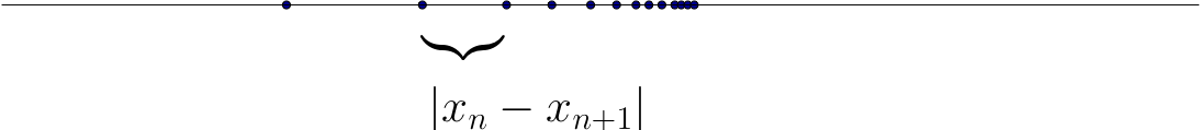
Cauchy Sequences

Informal definition: Cauchy sequences are those where $|x_n-x_{n+1}|$ gets smaller and smaller

Example

Sequences generated by iterative methods for solving nonlinear equations often have this property

Show code cell source Hide code cell source

f = lambda x: -4*x**3+5*x+1
g = lambda x: -12*x**2+5

def newton(fun,grad,x0,tol=1e-6,maxiter=100,callback=None):
    '''Newton method for solving equation f(x)=0
    with given tolerance and number of iterations.
    Callback function is invoked at each iteration if given.
    '''
    for i in range(maxiter):
        x1 = x0 - fun(x0)/grad(x0)
        err = abs(x1-x0)
        if callback != None: callback(err=err,x0=x0,x1=x1,iter=i)
        if err<tol: break
        x0 = x1
    else:
        raise RuntimeError('Failed to converge in %d iterations'%maxiter)
    return (x0+x1)/2

def print_err(iter,err,**kwargs):
    x = kwargs['x'] if 'x' in kwargs.keys() else kwargs['x0']
    print('{:4d}:  x = {:14.8f}    diff = {:14.10f}'.format(iter,x,err))

print('Newton method')
res = newton(f,g,x0=123.45,callback=print_err,tol=1e-10)

Newton method
   0:  x =   123.45000000    diff =  41.1477443465
   1:  x =    82.30225565    diff =  27.4306976138
   2:  x =    54.87155804    diff =  18.2854286376
   3:  x =    36.58612940    diff =  12.1877193931
   4:  x =    24.39841001    diff =   8.1212701971
   5:  x =    16.27713981    diff =   5.4083058492
   6:  x =    10.86883396    diff =   3.5965889909
   7:  x =     7.27224497    diff =   2.3839931063
   8:  x =     4.88825187    diff =   1.5680338561
   9:  x =     3.32021801    diff =   1.0119341175
  10:  x =     2.30828389    diff =   0.6219125117
  11:  x =     1.68637138    diff =   0.3347943714
  12:  x =     1.35157701    diff =   0.1251775194
  13:  x =     1.22639949    diff =   0.0188751183
  14:  x =     1.20752437    diff =   0.0004173878
  15:  x =     1.20710698    diff =   0.0000002022
  16:  x =     1.20710678    diff =   0.0000000000

Cauchy sequences “look like” they are converging to something

A key axiom of analysis is that such sequences do converge to something — details follow

Definition

A sequence $\{x_n\}$ is called Cauchy if $\mathrm{\forall }ϵ>0,\mathrm{\exists }N\in \mathbb{N}$ such that

$$n\ge N\text{ and }\mathrm{\forall }j\ge 1⟹|x_n-x_{n+j}|<ϵ$$

Example

$\{x_n\}$ defined by $x_n={\alpha }^n$ where $\alpha \in (0,1)$ is Cauchy

Proof

For any $n,j$ we have

$$|x_n-x_{n+j}|=|{\alpha }^n-{\alpha }^{n+j}|={\alpha }^n|1-{\alpha }^j|\le {\alpha }^n$$

Fix $ϵ>0$

We can show that $n>\log (ϵ)/\log (\alpha )⟹{\alpha }^n<ϵ$

Hence any integer $N>\log (ϵ)/\log (\alpha )$ the sequence is Cauchy by definition.

Fact

For any sequence the following equivalence holds: convergent $⟺$ Cauchy

Proof

Proof of $⟹$:

Let $\{x_n\}$ be a sequence converging to some $a\in \mathbb{R}$

Fix $ϵ>0$

We can choose $N$ s.t.

$$n\ge N⟹|x_n-a|<\frac{ϵ}{2}$$

For this $N$ we have $n\ge N$ and $j\ge 1$ implies

$$|x_n-x_{n+j}|\le |x_n-a|+|x_{n+j}-a|<\frac{ϵ}{2}+\frac{ϵ}{2}=ϵ$$

Proof of $\Leftarrow$:

This is basically an axiom in the definition of $\mathbb{R}$

Either

1. We assume it, or

2. We assume something else that’s essentially equivalent

Implications:

• There are no “gaps” in the real line

• To check $\{x_n\}$ converges to something we just need to check Cauchy property

Fact

Every bounded monotone sequence in $\mathbb{R}$ is convergent

Sketch of the proof:

Suffices to show that $\{x_n\}$ is Cauchy

Suppose not

Then no matter how far we go down the sequence we can find another jump of size $ϵ>0$

Since monotone, all the jumps are in the same direction

But then $\{x_n\}$ not bounded — a contradiction

Full proof: See any text on analysis

Subsequences

Definition

A sequence $\{x_{n_k}\}$ is called a subsequence of $\{x_n\}$ if

1. $\{x_{n_k}\}$ is a subset of $\{x_n\}$

2. the indices $n_k$ are strictly increasing

Example

$$\{x_n\}=\{x_1,x_2,x_3,x_4,x_5,\dots \}$$

$$\{x_{n_k}\}=\{x_2,x_4,x_6,x_8\dots \}$$

In this case

$$\{n_k\}=\{n_1,n_2,n_3,\dots \}=\{2,4,6,\dots \}$$

Example

$\{\frac{1}{1},\frac{1}{3},\frac{1}{5},\dots \}$ is a subsequence of $\{\frac{1}{1},\frac{1}{2},\frac{1}{3},\dots \}$

$\{\frac{1}{1},\frac{1}{2},\frac{1}{3},\dots \}$ is a subsequence of $\{\frac{1}{1},\frac{1}{2},\frac{1}{3},\dots \}$

$\{\frac{1}{2},\frac{1}{2},\frac{1}{2},\dots \}$ is not a subsequence of $\{\frac{1}{1},\frac{1}{2},\frac{1}{3},\dots \}$

Fact

Every sequence has a monotone subsequence

Proof omitted

Example

The sequence $x_n=(-1{)}^n$ has monotone subsequence

$$\{x_2,x_4,x_6,\dots \}=\{1,1,1,\dots \}$$

This leads us to the famous Bolzano-Weierstrass theorem, to be used later when we discuss optimization.

Fact: Bolzano-Weierstrass theorem

Every bounded sequence in $\mathbb{R}$ has a convergent subsequence

Proof

Let $\{x_n\}$ be a bounded sequence

There exists a monotone subsequence

• which is itself a bounded sequence (why?)

• and hence both monotone and bounded

Every bounded monotone sequence converges

Hence $\{x_n\}$ has a convergent subsequence

Derivatives

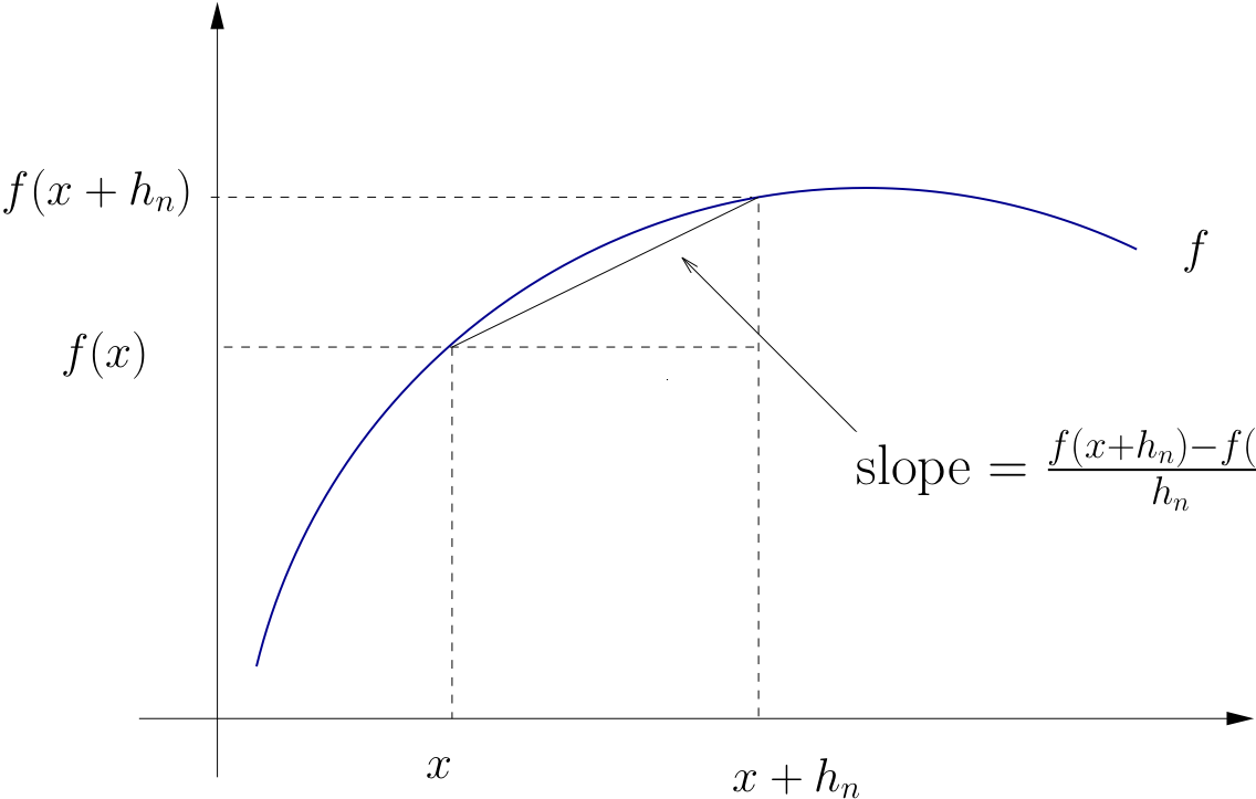
Definition

Let $f:(a,b)\to \mathbb{R}$ and let $x\in (a,b)$

Let $H$ be all sequences $\{h_n\}$ such that $h_n\ne 0$ and $h_n\to 0$

If there exists a constant $f^{\prime }(x)$ such that

$$\frac{f(x+h_n)-f(x)}{h_n}\to f^{\prime }(x)$$

for every $\{h_n\}\in H$, then

• $f$ is said to be differentiable at $x$

• $f^{\prime }(x)$ is called the derivative of $f$ at $x$

Example

Let $f:\mathbb{R}\to \mathbb{R}$ be defined by $f(x)=x^2$

Fix any $x\in \mathbb{R}$ and any $h_n\to 0$ with $n\to \mathrm{\infty }$

We have

$$\frac{f(x+h_n)-f(x)}{h_n}=\frac{(x+h_n{)}^2-x^2}{h_n}=$$

$$=\frac{x^2+2x{h}_n+h_n^2-x^2}{h_n}=2x+h_n$$

$$\text{therefore }{f}^{\prime }(x)=\underset{n\to \mathrm{\infty }}{lim}(2x+h_n)=2x$$

Example

Let $f:\mathbb{R}\to \mathbb{R}$ be defined by $f(x)=|x|$

This function is not differentiable at $x=0$

Indeed, if $h_n=1/n$, then

$$\frac{f(0+h_n)-f(0)}{h_n}=\frac{|0+1/n|-|0|}{1/n}\to 1$$

On the other hand, if $h_n=-1/n$, then

$$\frac{f(0+h_n)-f(0)}{h_n}=\frac{|0-1/n|-|0|}{-1/n}\to -1$$

Taylor series

Loosely speaking, if $f:\mathbb{R}\to \mathbb{R}$ is suitably differentiable at $a$, then

$$f(x)\approx f(a)+f^{\prime }(a)(x-a)$$

for $x$ very close to $a$,

$$f(x)\approx f(a)+f^{\prime }(a)(x-a)+\frac{f^{″}(a)}{2!}(x-a{)}^2$$

on a slightly wider interval, etc.

These are the 1st and 2nd order Taylor series approximations to $f$ at $a$ respectively

As the order goes higher we get better approximation

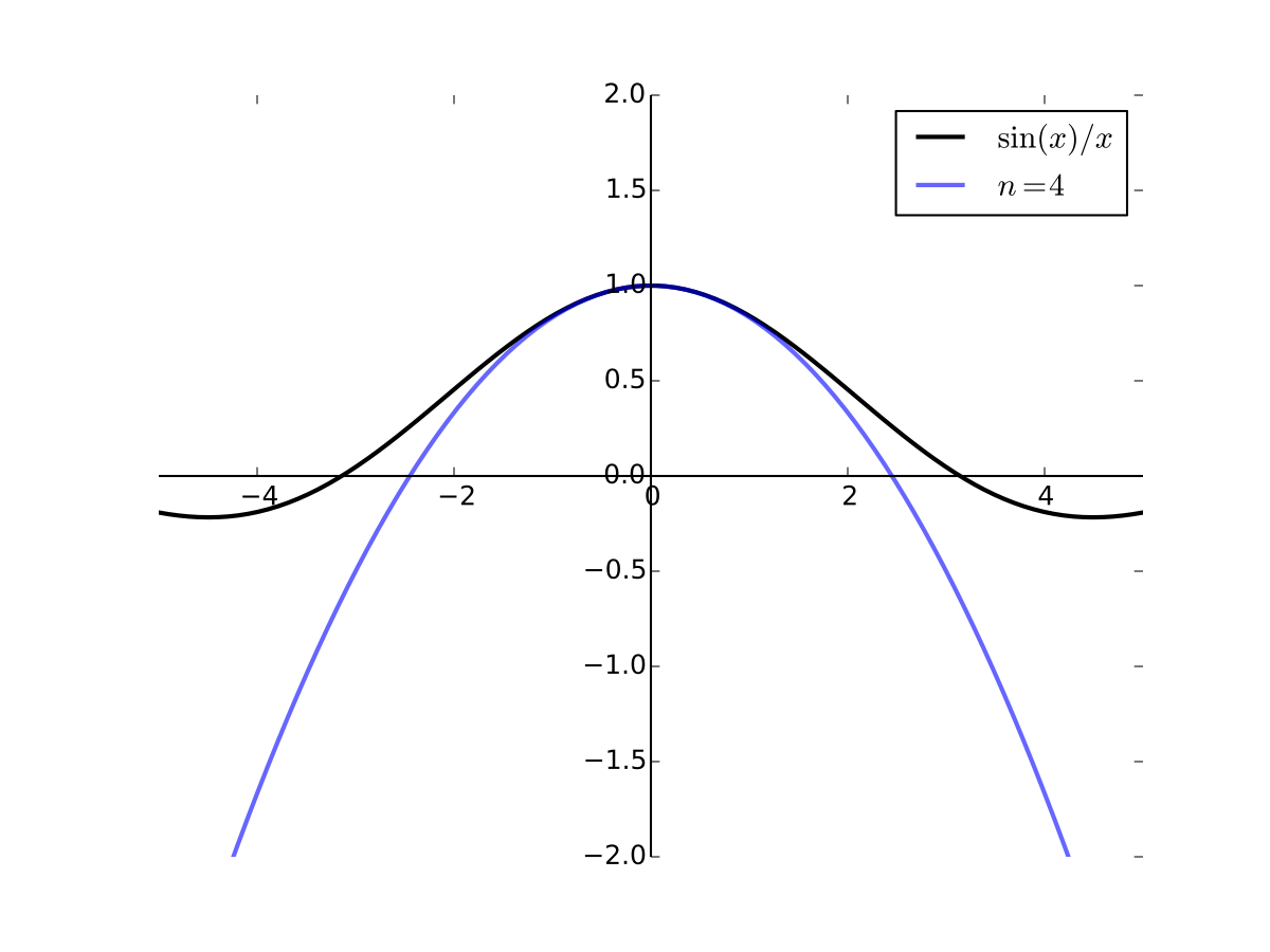
Fig. 33 4th order Taylor series for $f(x)=\sin (x)/x$ at 0

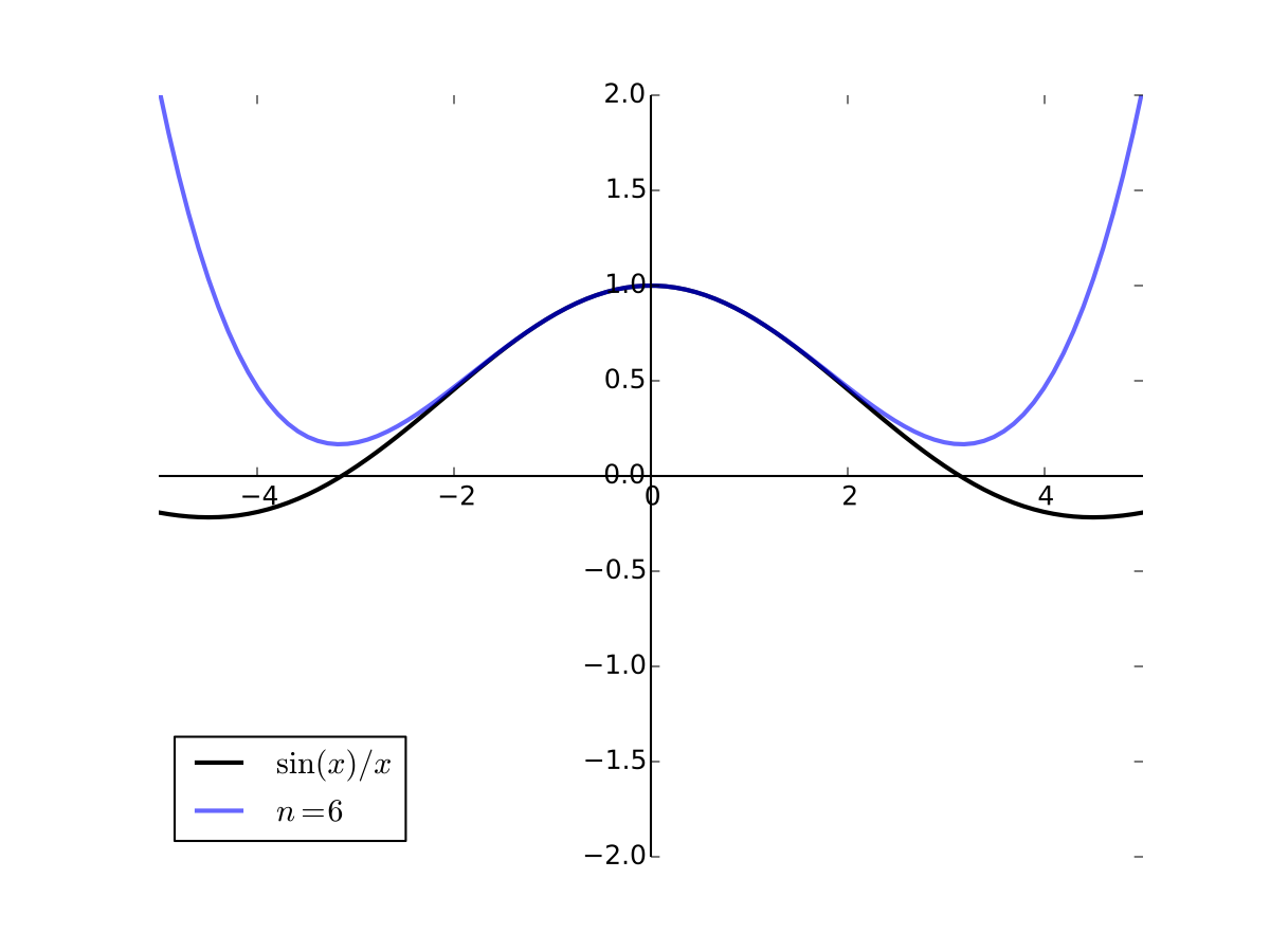
Fig. 34 6th order Taylor series for $f(x)=\sin (x)/x$ at 0

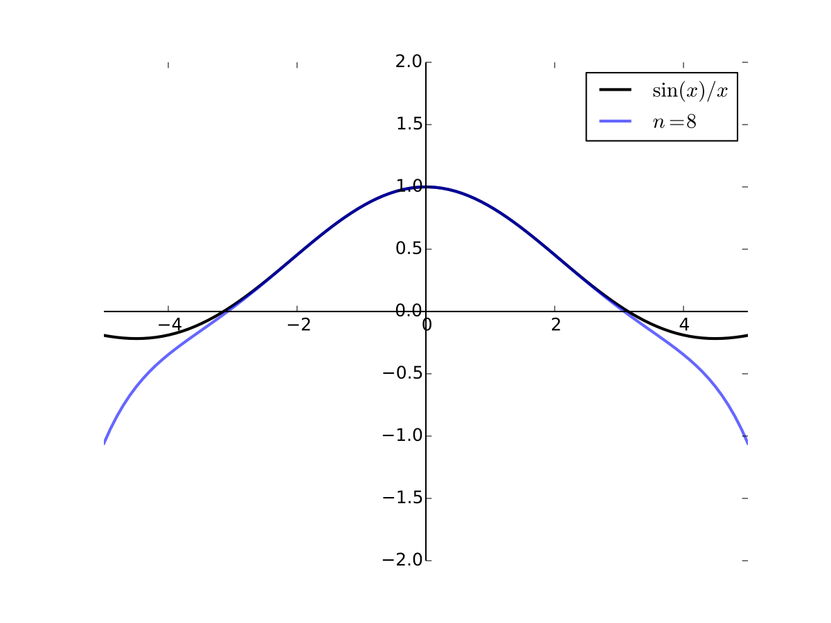
Fig. 35 8th order Taylor series for $f(x)=\sin (x)/x$ at 0

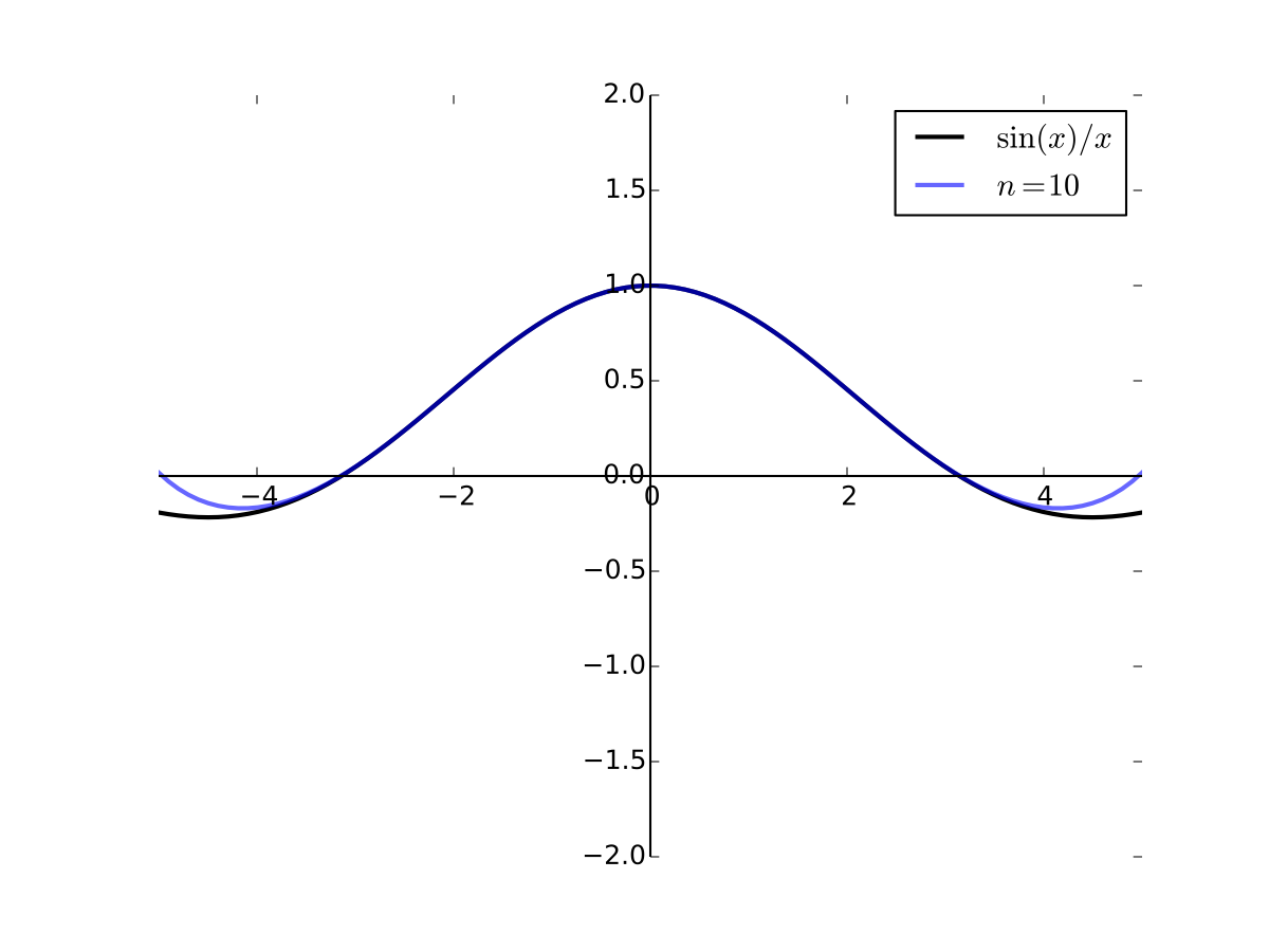
Fig. 36 10th order Taylor series for $f(x)=\sin (x)/x$ at 0

Analysis in ${\mathbb{R}}^K$

Now we switch from studying points $x\in \mathbb{R}$ to vectors $\mathbf{x}\in {\mathbb{R}}^K$

• Replace distance $|x-y|$ with $\Vert \mathbf{x}-\mathbf{y}\Vert$

Many of the same results go through otherwise unchanged

We state the analogous results briefly since

• You already have the intuition from $\mathbb{R}$

• Similar arguments, just replacing $|\cdot |$ with $\Vert \cdot \Vert$

We’ll spend longer on things that are different

Norm and distance

Definition

The (Euclidean) norm of $\mathbf{x}\in {\mathbb{R}}^N$ is defined as

$$\Vert \mathbf{x}\Vert :=\sqrt{{\mathbf{x}}^{\prime }\mathbf{x}}={\left(\sum _{n=1}^N{x}_n^2\right)}^{1/2}$$

Interpretation:

• $\Vert \mathbf{x}\Vert$ represents the length of $\mathbf{x}$

• $\Vert \mathbf{x}-\mathbf{y}\Vert$ represents distance between $\mathbf{x}$ and $\mathbf{y}$

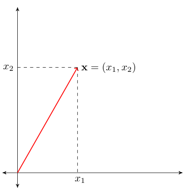
Fig. 37 Length of red line $=\sqrt{x_1^2+x_2^2}=:\Vert \mathbf{x}\Vert$

$\Vert \mathbf{x}-\mathbf{y}\Vert$ represents distance between $\mathbf{x}$ and $\mathbf{y}$

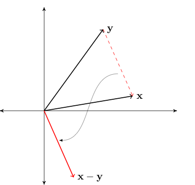
Fig. 38 Length of red line $=\Vert \mathbf{x}-\mathbf{y}\Vert$

Fact

For any $\alpha \in \mathbb{R}$ and any $\mathbf{x},\mathbf{y}\in {\mathbb{R}}^N$, the following statements are true:

• $\Vert \mathbf{x}\Vert \ge 0$ and $\Vert \mathbf{x}\Vert =0$ if and only if $\mathbf{x}=\mathbf{0}$

• $\Vert \alpha \mathbf{x}\Vert =|\alpha |\Vert \mathbf{x}\Vert$

• $\Vert \mathbf{x}+\mathbf{y}\Vert \le \Vert \mathbf{x}\Vert +\Vert \mathbf{y}\Vert$ (triangle inequality)

• $|{\mathbf{x}}^{\prime }\mathbf{y}|\le \Vert \mathbf{x}\Vert \Vert \mathbf{y}\Vert$ (Cauchy-Schwarz inequality)

For example, let’s show that $\Vert \mathbf{x}\Vert =0⟺\mathbf{x}=\mathbf{0}$

First let’s assume that $\Vert \mathbf{x}\Vert =0$ and show $\mathbf{x}=\mathbf{0}$

Since $\Vert \mathbf{x}\Vert =0$ we have $\Vert \mathbf{x}{\Vert }^2=0$ and hence $\sum _{n=1}^N{x}_n^2=0$

That is $x_n=0$ for all $n$, or, equivalently, $\mathbf{x}=\mathbf{0}$

Next let’s assume that $\mathbf{x}=\mathbf{0}$ and show $\Vert \mathbf{x}\Vert =0$

This is immediate from the definition of the norm

Bounded sets and $ϵ$-balls

Definition

A set $A\subset {\mathbb{R}}^K$ called bounded if

$$\mathrm{\exists }M\in \mathbb{R}\mathrm{such}\mathrm{that}\Vert \mathbf{x}\Vert \le M,\mathrm{\forall }\mathbf{x}\in A$$

Remarks:

• A generalization of the scalar definition

• When $K=1$, the norm $\Vert \cdot \Vert$ reduces to $|\cdot |$

Fact

If $A$ and $B$ are bounded sets then so is $C:=A\cup B$

Proof: Same as the scalar case — just replace $|\cdot |$ with $\Vert \cdot \Vert$

Exercise: Check it

Definition

For $ϵ>0$, the $ϵ$-ball $B_{ϵ}(\mathbf{a})$ around $\mathbf{a}\in {\mathbb{R}}^K$ is all $\mathbf{x}\in {\mathbb{R}}^K$ such that $\Vert \mathbf{a}-\mathbf{x}\Vert <ϵ$

Fact

If $\mathbf{x}$ is in every $ϵ$-ball around $\mathbf{a}$ then $\mathbf{x}=\mathbf{a}$

Fact

If $\mathbf{a}\ne \mathbf{b}$, then $\mathrm{\exists }ϵ>0$ such that $B_{ϵ}(\mathbf{a})\cap B_{ϵ}(\mathbf{b})=\mathrm{\varnothing }$

Definition

A sequence $\{{\mathbf{x}}_n\}$ in ${\mathbb{R}}^K$ is a function from $\mathbb{N}$ to ${\mathbb{R}}^K$

Definition

Sequence $\{{\mathbf{x}}_n\}$ is said to converge to $\mathbf{a}\in {\mathbb{R}}^K$ if

$$\mathrm{\forall }ϵ>0,\mathrm{\exists }N\in \mathbb{N}\text{ such that }n\ge N⟹{\mathbf{x}}_n\in B_{ϵ}(\mathbf{a})$$

We say: “$\{{\mathbf{x}}_n\}$ is eventually in any $ϵ$-neighborhood of $\mathbf{a}$”

In this case $\mathbf{a}$ is called the limit of the sequence, and we write

$${\mathbf{x}}_n\to \mathbf{a}\text{ as }n\to \mathrm{\infty }\text{or}\underset{n\to \mathrm{\infty }}{lim}{\mathbf{x}}_n=\mathbf{a}$$

Definition

We call $\{{\mathbf{x}}_n\}$ convergent if it converges to some limit in ${\mathbb{R}}^K$

Vector vs Componentwise Convergence

Fact

A sequence $\{{\mathbf{x}}_n\}$ in ${\mathbb{R}}^K$ converges to $\mathbf{a}\in {\mathbb{R}}^K$ if and only if each component sequence converges in $\mathbb{R}$

That is,

$$\begin{array}{r}\left(\begin{array}{c}{x}_n^1\\ ⋮\\ x_n^K\end{array}\right)\to \left(\begin{array}{c}{a}^1\\ ⋮\\ a^K\end{array}\right)\text{in }{\mathbb{R}}^K⟺\begin{array}{cc}{x}_n^1\to a^1& \text{in }\mathbb{R}\\ ⋮& \\ x_n^K\to a^K& \text{in }\mathbb{R}\end{array}\end{array}$$

From Scalar to Vector Analysis

More definitions analogous to scalar case:

Definition

A sequence $\{{\mathbf{x}}_n\}$ is called Cauchy if

$$\mathrm{\forall }ϵ>0,\mathrm{\exists }N\in \mathbb{N}\mathrm{such}\mathrm{that}n,m\ge N⟹\Vert {\mathbf{x}}_n-{\mathbf{x}}_m\Vert <ϵ$$

Definition

A sequence $\{{\mathbf{x}}_{n_k}\}$ is called a subsequence of $\{{\mathbf{x}}_n\}$ if

1. $\{{\mathbf{x}}_{n_k}\}$ is a subset of $\{{\mathbf{x}}_n\}$

2. the indices $n_k$ are strictly increasing

Fact

Analogous to the scalar case,

1. ${\mathbf{x}}_n\to \mathbf{a}$ in ${\mathbb{R}}^K$ if and only if $\Vert {\mathbf{x}}_n-\mathbf{a}\Vert \to 0$ in $\mathbb{R}$

2. If ${\mathbf{x}}_n\to \mathbf{x}$ and ${\mathbf{y}}_n\to \mathbf{y}$ then ${\mathbf{x}}_n+{\mathbf{y}}_n\to \mathbf{x}+\mathbf{y}$

3. If ${\mathbf{x}}_n\to \mathbf{x}$ and $\alpha \in \mathbb{R}$ then $\alpha {\mathbf{x}}_n\to \alpha \mathbf{x}$

4. If ${\mathbf{x}}_n\to \mathbf{x}$ and $\mathbf{z}\in {\mathbb{R}}^K$ then ${\mathbf{z}}^{\prime }{\mathbf{x}}_n\to {\mathbf{z}}^{\prime }\mathbf{x}$

5. Each sequence in ${\mathbb{R}}^K$ has at most one limit

6. Every convergent sequence in ${\mathbb{R}}^K$ is bounded

7. Every convergent sequence in ${\mathbb{R}}^K$ is Cauchy

8. Every Cauchy sequence in ${\mathbb{R}}^K$ is convergent

Exercise: Adapt proofs given for the scalar case to these results

Example

Let’s check that

$${\mathbf{x}}_n\to \mathbf{a}\text{ in }{\mathbb{R}}^K⟺\Vert {\mathbf{x}}_n-\mathbf{a}\Vert \to 0\text{ in }\mathbb{R}$$

Proof

• ${\mathbf{x}}_n\to \mathbf{a}$ in ${\mathbb{R}}^K$ means that

$$\mathrm{\forall }ϵ>0,\mathrm{\exists }N\in \mathbb{N}\mathrm{such}\mathrm{that}n\ge N⟹\Vert {\mathbf{x}}_n-\mathbf{a}\Vert <ϵ$$

• $\Vert {\mathbf{x}}_n-\mathbf{a}\Vert \to 0$ in $\mathbb{R}$ means that

$$\mathrm{\forall }ϵ>0,\mathrm{\exists }N\in \mathbb{N}\mathrm{such}\mathrm{that}n\ge N⟹|\Vert {\mathbf{x}}_n-\mathbf{a}\Vert -0|<ϵ$$

Obviously equivalent

Reminder — these facts are more general than scalar ones!

• True for any finite $K$

• So true for $K=1$

• This recovers the corresponding scalar fact

You can forget the scalar fact if you remember the vector one

Fact

If $\{{\mathbf{x}}_n\}$ converges to $\mathbf{x}$ in ${\mathbb{R}}^K$, then every subsequence of $\{{\mathbf{x}}_n\}$ also converges to $\mathbf{x}$

Fig. 39 Convergence of subsequences

Infinite Sums in ${\mathbb{R}}^K$

Analogous to the scalar case, an infinite sum in ${\mathbb{R}}^K$ is the limit of the partial sum

Definition

If $\{{\mathbf{x}}_n\}$ is a sequence in ${\mathbb{R}}^K$, then

$$\sum _{n=1}^{\mathrm{\infty }}{\mathbf{x}}_n:=\underset{J\to \mathrm{\infty }}{lim}\sum _{n=1}^J{\mathbf{x}}_n\text{ if the limit exists}$$

In other words,

$$\mathbf{y}=\sum _{n=1}^{\mathrm{\infty }}{\mathbf{x}}_n⟺\underset{J\to \mathrm{\infty }}{lim}\Vert \sum _{n=1}^J{\mathbf{x}}_n-\mathbf{y}\Vert \to 0$$

Open and Closed Sets

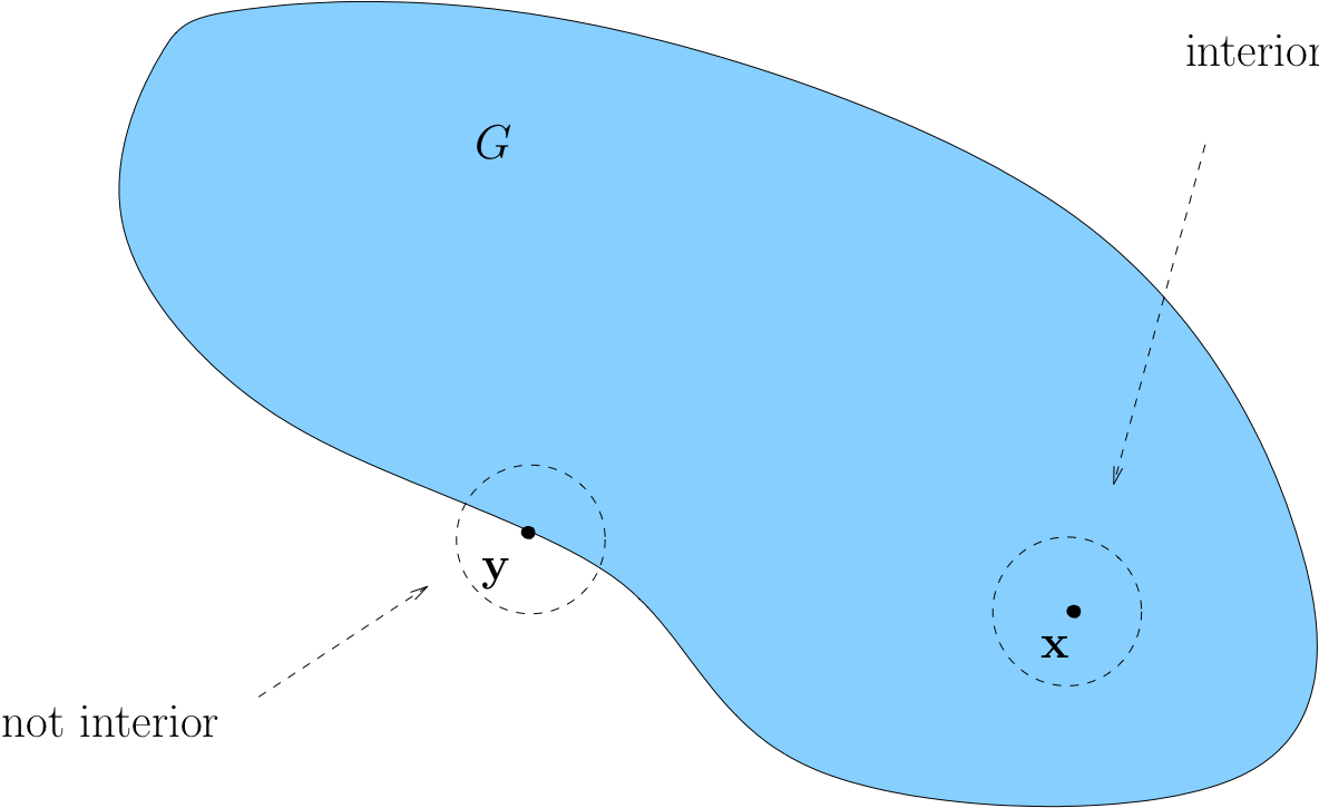
Let $G\subset {\mathbb{R}}^K$

Definition

We call $\mathbf{x}\in G$ interior to $G$ if $\mathrm{\exists }ϵ>0$ with $B_{ϵ}(\mathbf{x})\subset G$

Loosely speaking, interior means “not on the boundary”

Example

If $G=(a,b)$ for some $a<b$, then any $x\in (a,b)$ is interior

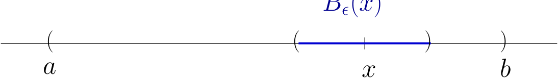
Proof

Fix any $a<b$ and any $x\in (a,b)$

Let $ϵ:=min\{x-a,b-x\}$

If $y\in B_{ϵ}(x)$ then $y<b$ because

$$y=y+x-x\le |y-x|+x<ϵ+x\le b-x+x=b$$

Exercise: Show $y\in B_{ϵ}(x)⟹y>a$

Example

If $G=[-1,1]$, then $1$ is not interior

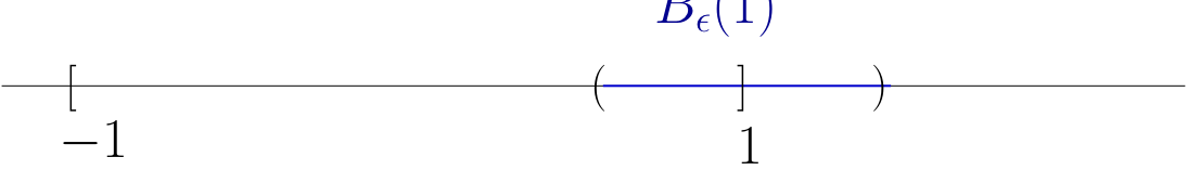
Intuitively, any $ϵ$-ball centered on $1$ will contain points $>1$

More formally, pick any $ϵ>0$ and consider $B_{ϵ}(1)$

There exists a $y\in B_{ϵ}(1)$ such that $y\notin [-1,1]$

For example, consider the point $y:=1+ϵ/2$

Exercise: Check this point: lies in $B_{ϵ}(1)$ but not in $[-1,1]$

Definition

A set $G\subset {\mathbb{R}}^K$ is called open if all of its points are interior

Example

Open sets:

• any “open” interval $(a,b)\subset \mathbb{R}$, since we showed all points are interior

• any “open” ball $B_{ϵ}(\mathbf{a})=\mathbf{x}\in {\mathbb{R}}^K:\Vert \mathbf{x}-\mathbf{a}\Vert <ϵ$

• ${\mathbb{R}}^K$ itself

Example

Sets that are not open

• $(a,b]$ because $b$ is not interior

• $[a,b)$ because $a$ is not interior

Closed Sets

Definition

A set $F\subset {\mathbb{R}}^K$ is called closed if every convergent sequence in $F$ converges to a point in $F$

Rephrased: If $\{{\mathbf{x}}_n\}\subset F$ and ${\mathbf{x}}_n\to \mathbf{x}$ for some $\mathbf{x}\in {\mathbb{R}}^K$, then $\mathbf{x}\in F$

Example

All of ${\mathbb{R}}^K$ is closed because every sequence converging to a point in ${\mathbb{R}}^K$ converges to a point in ${\mathbb{R}}^K$… right?

Example

If $(-1,1)\subset \mathbb{R}$ is not closed

Proof

True because

1. $x_n:=1-1/n$ is a sequence in $(-1,1)$ converging to $1$,

2. and yet $1\notin (-1,1)$

Example

If $F=[a,b]\subset \mathbb{R}$ then $F$ is closed in $\mathbb{R}$

Proof

Take any sequence $\{x_n\}$ such that

• $x_n\in F$ for all $n$

• $x_n\to x$ for some $x\in \mathbb{R}$

We claim that $x\in F$

Recall that (weak) inequalities are preserved under limits:

• $x_n\le b$ for all $n$ and $x_n\to x$, so $x\le b$

• $x_n\ge a$ for all $n$ and $x_n\to x$, so $x\ge a$

therefore $x\in [a,b]=:F$

Example

Any “hyperplane” of the form

$$H=\{\mathbf{x}\in {\mathbb{R}}^K:{\mathbf{x}}^{\prime }\mathbf{a}=c\}$$

is closed

Proof

Fix $\mathbf{a}\in {\mathbb{R}}^K$ and $c\in \mathbb{R}$ and let $H$ be as above

Let $\{{\mathbf{x}}_n\}\subset H$ with ${\mathbf{x}}_n\to \mathbf{x}\in {\mathbb{R}}^K$

We claim that $\mathbf{x}\in H$

Since ${\mathbf{x}}_n\in H$ and ${\mathbf{x}}_n\to \mathbf{x}$ we have

$${\mathbf{x}}_n^{\prime }\mathbf{a}\to {\mathbf{x}}^{\prime }\mathbf{a}\text{ in }\mathbb{R}\text{and}{\mathbf{x}}_n^{\prime }\mathbf{a}=c\text{ for all }n$$

$$\text{therefore }{\mathbf{x}}^{\prime }\mathbf{a}=\underset{n}{lim}{\mathbf{x}}_n^{\prime }\mathbf{a}=\underset{n}{lim}c=c$$

$$\text{therefore }\mathbf{x}\in H$$

Properties of Open and Closed Sets

Fact

$G\subset {\mathbb{R}}^K$ is open $⟺G^c$ is closed

Proof

$⟹$

First prove necessity

Pick any $G$ and let $F:=G^c$

Suppose to the contrary that $G$ is open but $F$ is not closed, so

$\mathrm{\exists }$ a sequence $\{{\mathbf{x}}_n\}\subset F$ with limit $\mathbf{x}\notin F$

Then $\mathbf{x}\in G$, and since $G$ open, $\mathrm{\exists }ϵ>0$ such that $B_{ϵ}(\mathbf{x})\subset G$

Since ${\mathbf{x}}_n\to \mathbf{x}$ we can choose an $N\in \mathbb{N}$ with ${\mathbf{x}}_N\in B_{ϵ}(\mathbf{x})$

This contradicts ${\mathbf{x}}_n\in F$ for all $n$

$⟸$

Next prove sufficiency

Pick any closed $F$ and let $G:=F^c$, need to prove that $G$ is open

Suppose to the contrary that $G$ is not open

Then exists some non-interior $\mathbf{x}\in G$, that is no $ϵ$-ball around $x$ lies entirely in $G$

Then it is possible to find a sequence $\{{\mathbf{x}}_n\}$ which converges to $x\in G$, but every element of which lies in the $B_{1/n}(\mathbf{x})\cap F$

This contradicts the fact that $F$ is closed

Example

Any singleton $\{\mathbf{x}\}\subset {\mathbb{R}}^K$ is closed

Proof

Let’s prove this by showing that $\{\mathbf{x}{\}}^c$ is open

Pick any $\mathbf{y}\in \{\mathbf{x}{\}}^c$

We claim that $\mathbf{y}$ is interior to $\{\mathbf{x}{\}}^c$

Since $\mathbf{y}\in \{\mathbf{x}{\}}^c$ it must be that $\mathbf{y}\ne \mathbf{x}$

Therefore, exists $ϵ>0$ such that $B_{ϵ}(\mathbf{y})\cap B_{ϵ}(\mathbf{x})=\mathrm{\varnothing }$

In particular, $\mathbf{x}\notin B_{ϵ}(\mathbf{y})$, and hence $B_{ϵ}(\mathbf{y})\subset \{\mathbf{x}{\}}^c$

Therefore $\mathbf{y}$ is interior as claimed

Since $\mathbf{y}$ was arbitrary it follows that $\{\mathbf{x}{\}}^c$ is open and $\{\mathbf{x}\}$ is closed

Fact

1. Any union of open sets is open

2. Any intersection of closed sets is closed

Proof

Proof of first fact:

Let $G:={\cup }_{\lambda \in \mathrm{\Lambda }}{G}_{\lambda }$, where each $G_{\lambda }$ is open

We claim that any given $\mathbf{x}\in G$ is interior to $G$

Pick any $\mathbf{x}\in G$

By definition, $\mathbf{x}\in G_{\lambda }$ for some $\lambda$

Since $G_{\lambda }$ is open, $\mathrm{\exists }ϵ>0$ such that $B_{ϵ}(\mathbf{x})\subset G_{\lambda }$

But $G_{\lambda }\subset G$, so $B_{ϵ}(\mathbf{x})\subset G$ also holds

In other words, $\mathbf{x}$ is interior to $G$

But be careful:

• An infinite intersection of open sets is not necessarily open

• An infinite union of closed sets is not necessarily closed

For example, if $G_n:=(-1/n,1/n)$, then ${\cap }_{n\in \mathbb{N}}{G}_n=\{0\}$

To see this, suppose that $x\in {\cap }_n{G}_n$

Then

$$-1/n<x<1/n,\mathrm{\forall }n\in \mathbb{N}$$

Therefore $x=0$, and hence $x\in \{0\}$

On the other hand, if $x\in \{0\}$ then $x\in {\cap }_n{G}_n$

Fact

If $A$ is closed and bounded then every sequence in $A$ has a subsequence which converges to a point of $A$

Take any sequence $\{{\mathbf{x}}_n\}$ contained in $A$

Since $A$ is bounded, $\{{\mathbf{x}}_n\}$ is bounded

Therefore it has a convergent subsequence

Since the subsequence is also contained in $A$, and $A$ is closed, the limit must lie in $A$.

Definition

Bounded and closed sets are called compact sets or compacts

Continuity

One of the most fundamental properties of functions

Related to existence of

• optima

• roots

• fixed points

• etc

as well as a variety of other useful concepts

Definition

A function $F$ is called bounded if its range is a bounded set.

Fact

If $F$ and $G$ are bounded, then so are $F+G$, $F\cdot G$ and $\alpha F$ for any finite $\alpha$

Proof

Proof for the case $F+G$:

Let $F$ and $G$ be bounded functions

$\mathrm{\exists }$ $M_F$ and $M_G$ s.t. $\Vert F(\mathbf{x})\Vert \le M_F$ and $\Vert G(\mathbf{x})\Vert \le M_G$ for all $\mathbf{x}$

Fix any $\mathbf{x}$ and let $M:=M_F+M_G$

Applying the triangle inequality gives

$$\Vert (F+G)(\mathbf{x})\Vert :=\Vert F(\mathbf{x})+G(\mathbf{x})\Vert \le \Vert F(\mathbf{x})\Vert +\Vert G(\mathbf{x})\Vert \le M$$

Since $\mathbf{x}$ was arbitrary this bound holds for all $\mathbf{x}$

Let $F:A\to {\mathbb{R}}^J$ where $A$ is a subset of ${\mathbb{R}}^K$

Definition

$F$ is called continuous at $\mathbf{x}\in A$ if as $n\to \mathrm{\infty }$

$${\mathbf{x}}_n\to \mathbf{x}⟹F({\mathbf{x}}_n)\to F(\mathbf{x})$$

Requires that

• $F({\mathbf{x}}_n)$ converges for each choice of ${\mathbf{x}}_n\to \mathbf{x}$,

• The limit is always the same, and that limit is $F(\mathbf{x})$

Definition

$F$ is called continuous if it is continuous at every $\mathbf{x}\in A$

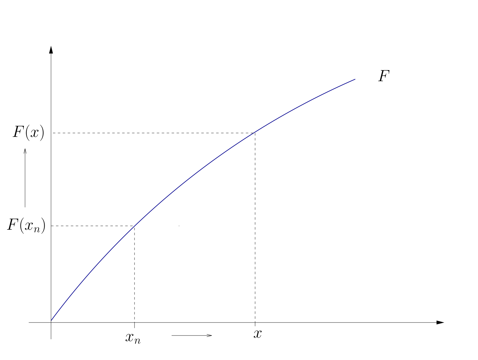
Fig. 40 Continuity

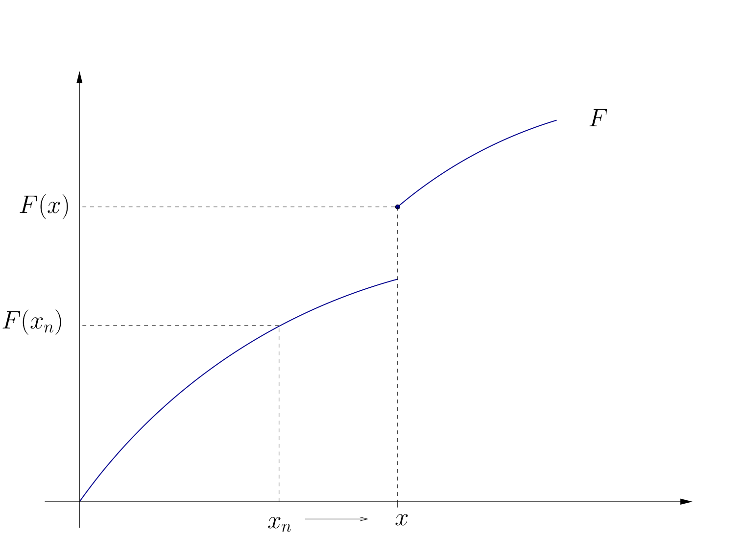
Fig. 41 Discontinuity at $x$

Example

Let $\mathbf{A}$ be an $J\times K$ matrix and let $F(\mathbf{x})=\mathbf{A}\mathbf{x}$

The function $F$ is continuous at every $\mathbf{x}\in {\mathbb{R}}^K$

To see this take

• any $\mathbf{x}\in {\mathbb{R}}^K$

• any ${\mathbf{x}}_n\to \mathbf{x}$

By the definition of the matrix norm $\Vert \mathbf{A}\Vert$, we have

$$\Vert \mathbf{A}{\mathbf{x}}_n-\mathbf{A}\mathbf{x}\Vert =\Vert \mathbf{A}({\mathbf{x}}_n-\mathbf{x})\Vert \le \Vert \mathbf{A}\Vert \Vert {\mathbf{x}}_n-\mathbf{x}\Vert$$

$$\text{therefore }{\mathbf{x}}_n\to \mathbf{x}⟹\mathbf{A}{\mathbf{x}}_n\to \mathbf{A}\mathbf{x}$$

Exercise: Exactly what rules are we using here?

Fact

If $f:\mathbb{R}\to \mathbb{R}$ is differentiable at $x$, then $f$ is continuous at $x$

Fact

Some functions known to be continuous on their domains:

• $x\mapsto x^{\alpha }$

• $x\mapsto |x|$

• $x\mapsto \log (x)$

• $x\mapsto \exp (x)$

• $x\mapsto \sin (x)$

• $x\mapsto \cos (x)$

Example

Discontinuous at zero: $x\mapsto \mathbb{1}\{x>0\}$.

Fact

Let $F$ and $G$ be functions and let $\alpha \in \mathbb{R}$

1. If $F$ and $G$ are continuous at $\mathbf{x}$ then so is $F+G$, where

$$(F+G)(\mathbf{x}):=F(\mathbf{x})+G(\mathbf{x})$$

2. If $F$ is continuous at $\mathbf{x}$ then so is $\alpha F$, where

$$(\alpha F)(\mathbf{x}):=\alpha F(\mathbf{x})$$

3. If $F$ and $G$ are continuous at $\mathbf{x}$ and real valued then so is $FG$, where

$$(FG)(\mathbf{x}):=F(\mathbf{x})\cdot G(\mathbf{x})$$

In the latter case, if in addition $G(\mathbf{x})\ne 0$, then $F/G$ is also continuous.

As a result, set of continuous functions is “closed” under elementary arithmetic operations

Example

The function $F:\mathbb{R}\to \mathbb{R}$ defined by

$$F(x)=\frac{\exp (x)+\sin (x)}{2+\cos (x)}+\frac{x^4}{2}-\frac{{\cos }^3(x)}{8!}$$

is continuous

Proof

Just repeatedly apply the rules on the previous slide

Let’s just check that

$$F\text{ and }G\text{ continuous at }\mathbf{x}⟹F+G\text{ continuous at }\mathbf{x}$$

Let $F$ and $G$ be continuous at $\mathbf{x}$

Pick any ${\mathbf{x}}_n\to \mathbf{x}$

We claim that $F({\mathbf{x}}_n)+G({\mathbf{x}}_n)\to F(\mathbf{x})+G(\mathbf{x})$

By assumption, $F({\mathbf{x}}_n)\to F(\mathbf{x})$ and $G({\mathbf{x}}_n)\to G(\mathbf{x})$

From this and the triangle inequality we get

$$\Vert F({\mathbf{x}}_n)+G({\mathbf{x}}_n)-(F(\mathbf{x})+G(\mathbf{x}))\Vert \le$$

$$\le \Vert F({\mathbf{x}}_n)-F(\mathbf{x})\Vert +\Vert G({\mathbf{x}}_n)-G(\mathbf{x})\Vert \to 0$$

Extra material

Watch excellent video by Grant Sanderson (3blue1brown) on limits, and continue onto his whole amazing series on calculus