Univariate and bivariate optimization

ECON2125/6012 Lecture 2 Fedor Iskhakov

Announcements & Reminders

• Tutorials start tomorrow (Aug 4)

• Register for tutorials on Wattle if you have not done so already

• Office hours of the tutors are updated:

  • Wending Liu

    • Email: Wending.Liu@anu.edu.au

    • Room: Room 2084, Copland Bld (24) (updated!)

    • Office hours: Friday 1pm-3pm

  • Chien Yeh

    • Email: Chien.Yeh@anu.edu.au

    • Room: Room 2106, Copland Bld (24)

    • Office hours: Monday 2pm-4pm

• Reminder on how to ask questions:

  1. Administrative: RSE admin

  2. Content/understanding: tutors

  3. Other: to Fedor

Plan for this lecture

1. Motivation (math vs. computing)

2. Univariate optimization

3. Working with bivariate functions

4. Bivariate optimization

Supplementary reading:

• Simon & Blume: part 1 (revision)

• Sundaram: sections 1.1, 1.4, chapter 2, chapter 4

Computing

The classic way we do mathematics is pencil and paper

In 1944, Hans Bethe solved following problem by hand:
Will detonating an atom bomb ignite the atmosphere and thereby destroy life on earth?
source

These days we rarely calculate with actual numbers

Almost all calculations are done on computers

Example: numerical integration

\[ \frac{1}{\sqrt{2\pi}} \int_{-2}^2 \exp\left\{ - \frac{x^2}{2} \right\} dx \]

from scipy.stats import norm
from scipy.integrate import quad
phi = norm()
value, error = quad(phi.pdf, -2, 2)
print('Integral value =',value)

Integral value = 0.9544997361036417

Example: Numerical optimization

\[ f(x) = - \exp \left\{-\frac{(x - 5.0)^4}{1.5} \right\} \rightarrow \min \]

from scipy.optimize import fminbound
import numpy as np
f = lambda x: -np.exp(-(x - 5.0)**4 / 1.5)
res = fminbound(f, -10, 10)  # find approx solution
print('Minimum value is attained approximately at', res)

Minimum value is attained approximately at 4.999941901210501

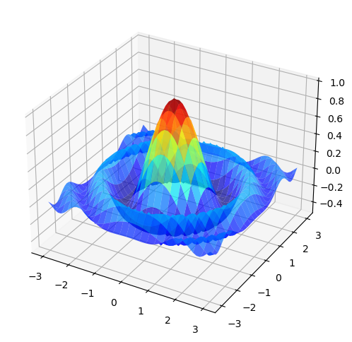
Example: Visualization

What does this function look like?

\[ f(x, y) = \frac{\cos(x^2 + y^2)}{1 + x^2 + y^2} \]

import matplotlib.pyplot as plt
from mpl_toolkits.mplot3d.axes3d import Axes3D
import numpy as np
from matplotlib import cm
f = lambda x, y: np.cos(x**2 + y**2) / (1 + x**2 + y**2)
xgrid = np.linspace(-3, 3, 50)
ygrid = xgrid
x, y = np.meshgrid(xgrid, ygrid)
fig = plt.figure(figsize=(8, 6))
ax = fig.add_subplot(111, projection='3d')
ax.plot_surface(x,
                y,
                f(x, y),
                rstride=2, cstride=2,
                cmap=cm.jet,
                alpha=0.7,
                linewidth=0.25)
ax.set_zlim(-0.5, 1.0)
plt.show()

Example: Symbolic calculations

Differentiate \(f(x) = (1 + 2x)^5\).
Forgotten how? No problems, just ask a computer for symbolic derivative

import sympy as sp
x = sp.Symbol('x')
fx = (1 + 2 * x)**5
print("Derivative of",fx,"is",fx.diff(x))

Derivative of (2*x + 1)**5 is 10*(2*x + 1)**4

So if computers can do our maths for us, why learn maths?

The difficulty is

• giving them the right inputs and instructions

• interpreting what comes out

The skills we need are

• Understanding of fundamental concepts

• Sound deductive reasoning

These are the focus of the course

Computer Code in the Lectures

While computation is not a formal part of the course
there will be little bits of code in the lectures to illustrate the kinds of things we can do.

• All the code will be written in the Python programming language

• It is not assessable

You might find value in actually running the code shown in lectures
If you want to do so please refer to linked GitHub repository in optim.iskh.me

Univariate Optimization

Let \(f \colon [a, b] \to \mathbb{R}\) be a differentiable (smooth) function

• \([a, b]\) is all \(x\) with \(a \leq x \leq b\)

• \(\mathbb{R}\) is “all numbers”

• \(f\) takes \(x \in [a, b]\) and returns number \(f(x)\)

• derivative \(f'(x)\) exists for all \(x\) with \(a < x < b\)

Definition

A point \(x^* \in [a, b]\) is called a

• maximizer of \(f\) on \([a, b]\) if \(f(x^*) \geq f(x)\) for all \(x \in [a,b]\)

• minimizer of \(f\) on \([a, b]\) if \(f(x^*) \leq f(x)\) for all \(x \in [a,b]\)

Show code cell content Hide code cell content

from myst_nb import glue
import matplotlib.pyplot as plt
import numpy as np

def subplots():
    "Custom subplots with axes through the origin"
    fig, ax = plt.subplots()
    # Set the axes through the origin
    for spine in ['left', 'bottom']:
        ax.spines[spine].set_position('zero')
    for spine in ['right', 'top']:
        ax.spines[spine].set_color('none')
    return fig, ax

xmin, xmax = 2, 8
xgrid = np.linspace(xmin, xmax, 200)
f = lambda x: -(x - 4)**2 + 10

xstar = 4.0
fig, ax = subplots()
ax.plot([xstar], [0],  'ro', alpha=0.6)
ax.set_ylim(-12, 15)
ax.set_xlim(-1, 10)
ax.set_xticks([2, xstar, 6, 8, 10])
ax.set_xticklabels([2, r'$x^*=4$', 6, 8, 10], fontsize=14)
ax.plot(xgrid, f(xgrid), 'b-', lw=2, alpha=0.8, label=r'$f(x) = -(x-4)^2+10$')
ax.plot((xstar, xstar), (0, f(xstar)), 'k--', lw=1, alpha=0.8)
#ax.legend(frameon=False, loc='upper right', fontsize=16)
glue("fig_maximizer", fig, display=False)

xstar = xmax
fig, ax = subplots()
ax.plot([xstar], [0],  'ro', alpha=0.6)
ax.text(xstar, 1, r'$x^{**}=8$', fontsize=16)
ax.set_ylim(-12, 15)
ax.set_xlim(-1, 10)
ax.set_xticks([2, 4, 6, 10])
ax.set_xticklabels([2, 4, 6, 10], fontsize=14)
ax.plot(xgrid, f(xgrid), 'b-', lw=2, alpha=0.8, label=r'$f(x) = -(x-4)^2+10$')
ax.plot((xstar, xstar), (0, f(xstar)), 'k--', lw=1, alpha=0.8)
#ax.legend(frameon=False, loc='upper right', fontsize=16)
glue("fig_minimizer", fig, display=False)

xmin, xmax = 0, 1
xgrid1 = np.linspace(xmin, xmax, 100)
xgrid2 = np.linspace(xmax, 2, 10)

fig, ax = subplots()
ax.set_ylim(0, 1.1)
ax.set_xlim(-0.0, 2)
func_string = r'$f(x) = x^2$ if $x < 1$ else $f(x) = 0.5$'
ax.plot(xgrid1, xgrid1**2, 'b-', lw=3, alpha=0.6, label=func_string)
ax.plot(xgrid2, 0 * xgrid2 + 0.5, 'b-', lw=3, alpha=0.6)
#ax.legend(frameon=False, loc='lower right', fontsize=16)
glue("fig_none", fig, display=False)

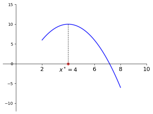
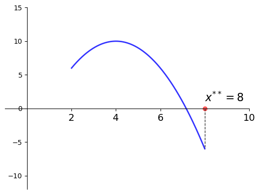
Example

Let

• \(f(x) = -(x-4)^2 + 10\)

• \(a = 2\) and \(b=8\)

Then

• \(x^* = 4\) is a maximizer of \(f\) on \([2, 8]\)

• \(x^{**} = 8\) is a minimizer of \(f\) on \([2, 8]\)

Fig. 1 Maximizer on \([a, b] = [2, 8]\) is \(x^* = 4\)

Fig. 2 Minimizer on \([a, b] = [2, 8]\) is \(x^{**} = 8\)

The set of maximizers/minimizers can be

• empty

• a singleton (contains one element)

• infinite (contains infinitely many elements)

Example: infinite maximizers

\(f \colon [0, 1] \to \mathbb{R}\) defined by \(f(x) =1\)
has infinitely many maximizers and minimizers on \([0, 1]\)

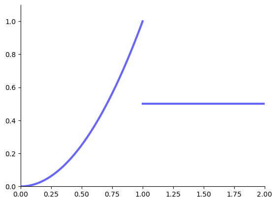
Example: no maximizers

The following function has no maximizers on \([0, 2]\)

\[\begin{split} f(x) = \begin{cases} x^2 & \text{ if } x < 1 \\ 1/2 & \text{ otherwise} \end{cases} \end{split}\]

Fig. 3 No maximizer on \([0, 2]\)

Definition

Point \(x\) is called interior to \([a, b]\) if \(a < x < b\)

The set of all interior points is written \((a, b)\)

We refer to \(x^* \in [a, b]\) as

• interior maximizer if both a maximizer and interior

• interior minimizer if both a minimizer and interior

Finding optima

Definition

A stationary point of \(f\) on \([a, b]\) is an interior point \(x\) with \(f'(x) = 0\)

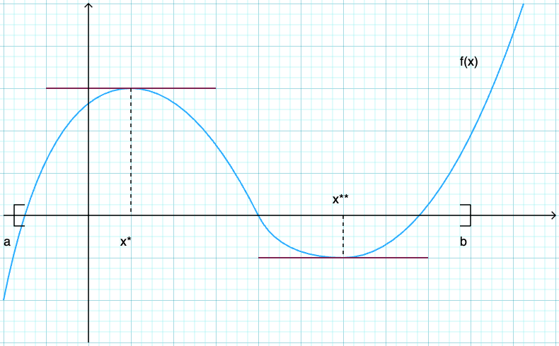
Fig. 4 Both \(x^*\) and \(x^{**}\) are stationary

Fact

If \(f\) is differentiable and \(x^*\) is either an interior minimizer or an interior maximizer of \(f\) on \([a, b]\), then \(x^*\) is stationary

Sketch of proof, for maximizers:

\[ f'(x^*) = \, \lim_{h \to 0} \, \frac{f(x^* + h) - f(x^*)}{h} \qquad \text{(by def.)} \]

\[ \Rightarrow f(x^* + h) \approx f(x^*) + f'(x^*) h \qquad \text{for small } h \]

If \(f'(x^*) \ne 0\) then exists small \(h\) such that \(f(x^* + h) > f(x^*)\)

Hence interior maximizers must be stationary — otherwise we can do better

\(\Rightarrow\) any interior maximizer stationary
\(\Rightarrow\) set of interior maximizers \(\subset\) set of stationary points
\(\Rightarrow\) maximizers \(\subset\) stationary points \(\cup \{a\} \cup \{b\}\)

Algorithm for univariate problems

1. Locate stationary points

2. Evaluate \(y = f(x)\) for each stationary \(x\) and for \(a\), \(b\)

3. Pick point giving largest \(y\) value

Minimization: same idea

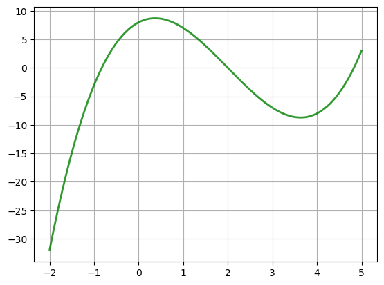
Example

Let’s solve

\[ \max_{-2 \leq x \leq 5} f(x) \quad \text{where} \quad f(x) = x^3 - 6x^2 + 4x + 8 \]

Steps

• Differentiate to get \(f'(x) = 3x^2 - 12x + 4\)

• Solve \(3x^2 - 12x + 4 = 0\) to get stationary \(x\)

• Discard any stationary points outside \([-2, 5]\)

• Eval \(f\) at remaining points plus end points \(-2\) and \(5\)

• Pick point giving largest value

from sympy import *
x = Symbol('x')
points = [-2, 5]
f = x**3 - 6*x**2 + 4*x + 8
fp = diff(f, x)
spoints = solve(fp, x)
points.extend(spoints)
v = [f.subs(x, c).evalf() for c in points]
maximizer = points[v.index(max(v))]
print("Maximizer =", str(maximizer),'=',maximizer.evalf())

Maximizer = 2 - 2*sqrt(6)/3 = 0.367006838144548

Show code cell source Hide code cell source

import matplotlib.pyplot as plt
import numpy as np
xgrid = np.linspace(-2, 5, 200)
f = lambda x: x**3 - 6*x**2 + 4*x + 8
fig, ax = plt.subplots()
ax.plot(xgrid, f(xgrid), 'g-', lw=2, alpha=0.8)
ax.grid()

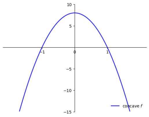
Shape Conditions and Sufficiency

When is \(f'(x^*) = 0\) sufficient for \(x^*\) to be a maximizer?

One answer: When \(f\) is concave

Show code cell source Hide code cell source

xgrid = np.linspace(-2, 2, 200)
f = lambda x: - 8*x**2 + 8
fig, ax = subplots()
ax.set_ylim(-15, 10)
ax.set_yticks([-15, -10, -5, 5, 10])
ax.set_xticks([-1, 0, 1])
ax.plot(xgrid, f(xgrid), 'b-', lw=2, alpha=0.8, label='concave $f$')
ax.legend(frameon=False, loc='lower right')
plt.show()

(Full definition deferred)

Sufficient conditions for concavity in one dimension

Let \(f \colon [a, b] \to \mathbb{R}\)

• If \(f''(x) \leq 0\) for all \(x \in (a, b)\) then \(f\) is concave on \((a, b)\)

• If \(f''(x) < 0\) for all \(x \in (a, b)\) then \(f\) is strictly concave on \((a, b)\)

Example

• \(f(x) = a + b x\) is concave on \(\mathbb{R}\) but not strictly

• \(f(x) = \log(x)\) is strictly concave on \((0, \infty)\)

When is \(f'(x^*) = 0\) sufficient for \(x^*\) to be a minimizer?

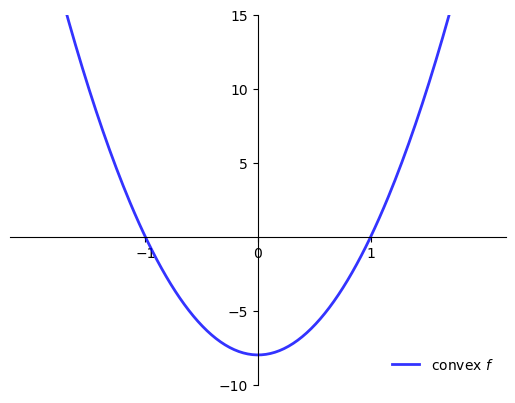
One answer: When \(f\) is convex

Show code cell source Hide code cell source

xgrid = np.linspace(-2, 2, 200)
f = lambda x: - 8*x**2 + 8
fig, ax = subplots()
ax.set_ylim(-10, 15)
ax.set_yticks([-10, -5, 5, 10, 15])
ax.set_xticks([-1, 0, 1])
ax.plot(xgrid, -f(xgrid), 'b-', lw=2, alpha=0.8, label='convex $f$')
ax.legend(frameon=False, loc='lower right')
plt.show()

(Full definition deferred)

Sufficient conditions for convexity in one dimension

Let \(f \colon [a, b] \to \mathbb{R}\)

• If \(f''(x) \geq 0\) for all \(x \in (a, b)\) then \(f\) is convex on \((a, b)\)

• If \(f''(x) > 0\) for all \(x \in (a, b)\) then \(f\) is strictly convex on \((a, b)\)

Example

• \(f(x) = a + b x\) is convex on \(\mathbb{R}\) but not strictly

• \(f(x) = x^2\) is strictly convex on \(\mathbb{R}\)

Sufficiency and uniqueness with shape conditions

Fact

For maximizers:

• If \(f \colon [a,b] \to \mathbb{R}\) is concave and \(x^* \in (a, b)\) is stationary then \(x^*\) is a maximizer

• If, in addition, \(f\) is strictly concave, then \(x^*\) is the unique maximizer

Fact

For minimizers:

• If \(f \colon [a,b] \to \mathbb{R}\) is convex and \(x^* \in (a, b)\) is stationary then \(x^*\) is a minimizer

• If, in addition, \(f\) is strictly convex, then \(x^*\) is the unique minimizer

Example

A price taking firm faces output price \(p > 0\), input price \(w >0\)

Maximize profits with respect to input \(\ell\)

\[ \max_{\ell \ge 0} \pi(\ell) = p f(\ell) - w \ell, \]

where the production technology is given by

\[ f(\ell) = \ell^{\alpha}, 0 < \alpha < 1. \]

Evidently

\[ \pi'(\ell) = \alpha p \ell^{\alpha - 1} - w, \]

so unique stationary point is

\[ \ell^* = (\alpha p/w)^{1/(1 - \alpha)} \]

Moreover,

\[ \pi''(\ell) = \alpha (\alpha - 1) p \ell^{\alpha - 2} < 0 \]

for all \(\ell \ge 0\) so \(\ell^*\) is unique maximizer.

Show code cell content Hide code cell content

p = 2.0
w = 1.0
alpha = 0.6
xstar = (alpha * p / w)**(1/(1 - alpha))
xgrid = np.linspace(0, 4, 200)
f = lambda x: x**alpha
pi = lambda x: p * f(x) - w * x
fig, ax = subplots()
ax.set_xticks([1,xstar,2,3])
ax.set_xticklabels(['1',r'$\ell^*$','2','3'], fontsize=14)
ax.plot(xgrid, pi(xgrid), 'b-', lw=2, alpha=0.8, label=r'$\pi(\ell) = p\ell^{\alpha} - w\ell$')
ax.plot((xstar, xstar), (0, pi(xstar)), 'g--', lw=1, alpha=0.8)
#ax.legend(frameon=False, loc='upper right', fontsize=16)
glue("fig_price_taker", fig, display=False)
glue("ellstar", round(xstar,4))

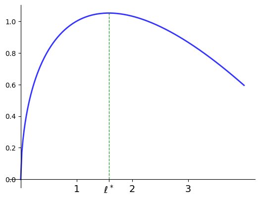
Fig. 5 Profit maximization with \(p=2\), \(w=1\), \(\alpha=0.6\), \(\ell^*=\)1.5774

Functions of two variables

Let’s have a look at some functions of two variables

• How to visualize them

• Slope, contours, etc.

Example: Cobb-Douglas production function

Consider production function

\[\begin{split} f(k, \ell) = k^{\alpha} \ell^{\beta}\\ \alpha \ge 0, \, \beta \ge 0, \, \alpha + \beta < 1 \end{split}\]

Let’s graph it in two dimensions.

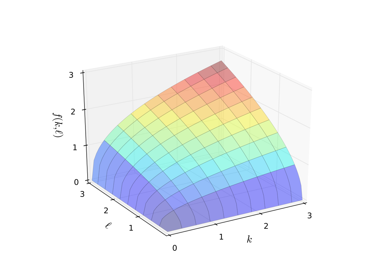
Fig. 6 Production function with \(\alpha=0.4\), \(\beta=0.5\) (a)

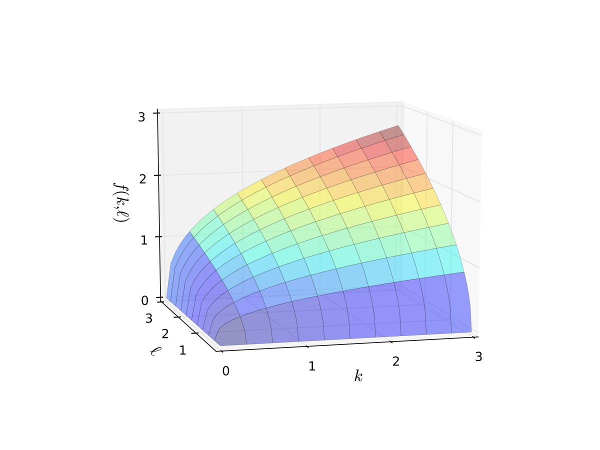
Fig. 7 Production function with \(\alpha=0.4\), \(\beta=0.5\) (b)

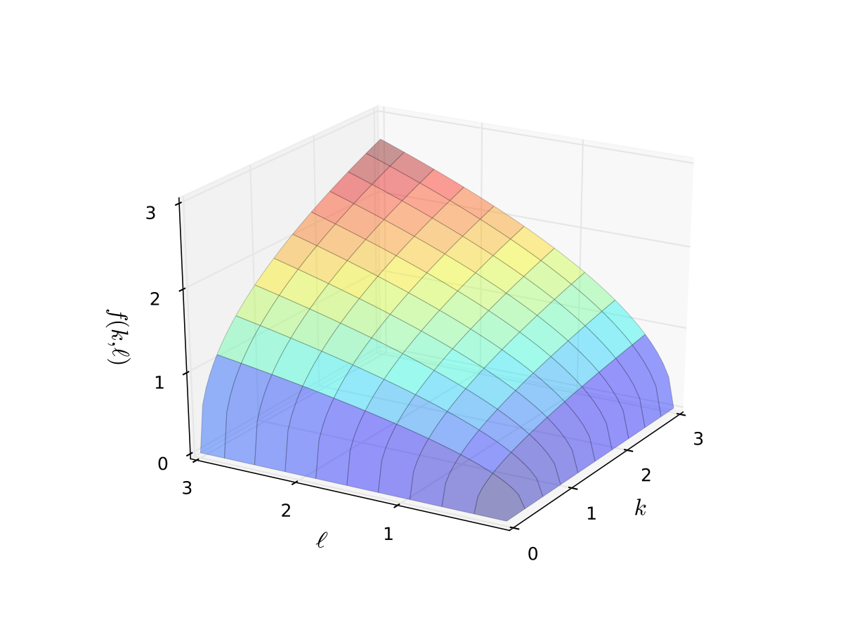
Fig. 8 Production function with \(\alpha=0.4\), \(\beta=0.5\) (c)

Like many 3D plots it’s hard to get a good understanding

Let’s try again with contours plus heat map

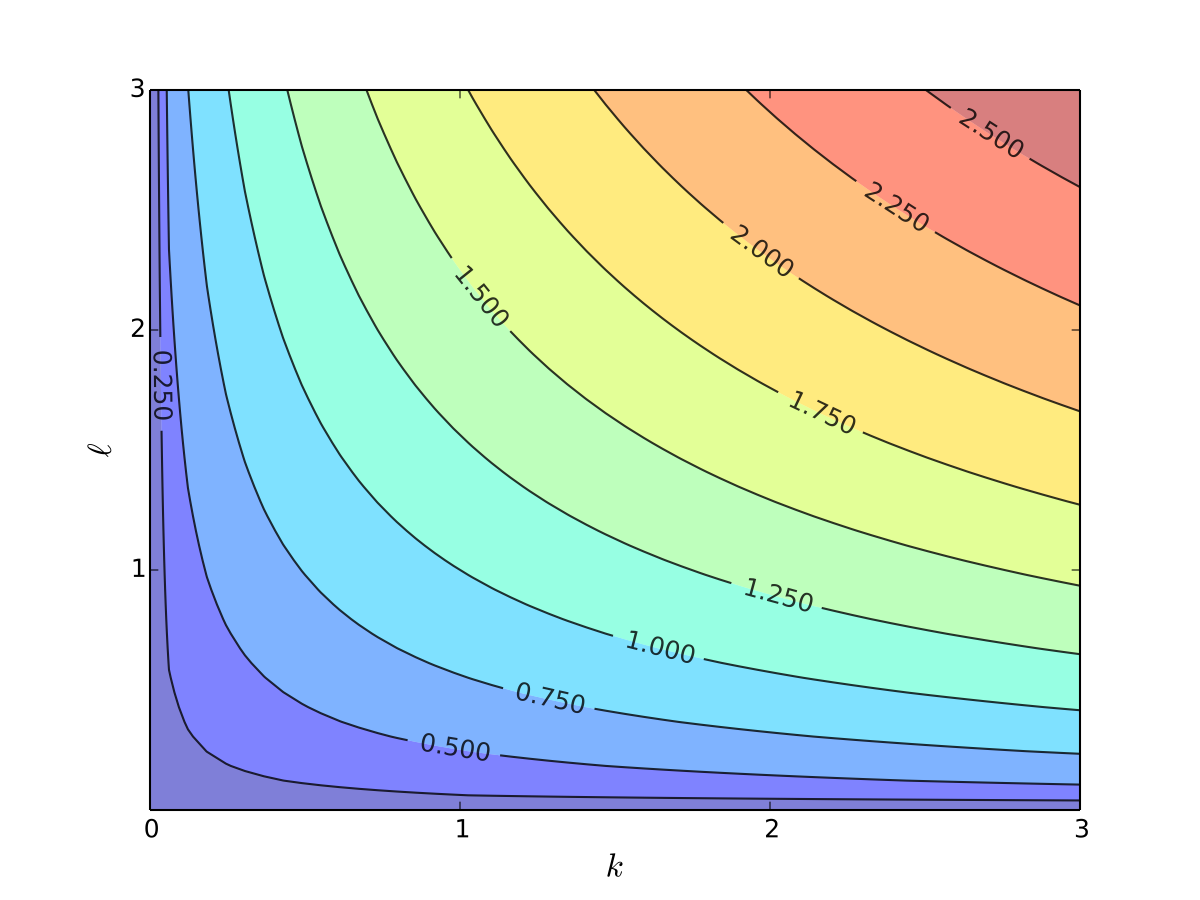
Fig. 9 Production function with \(\alpha=0.4\), \(\beta=0.5\), contours

In this context the contour lines are called isoquants

Can you see how \(\alpha < \beta\) shows up in the slope of the contours?

We can drop the colours to see the numbers more clearly

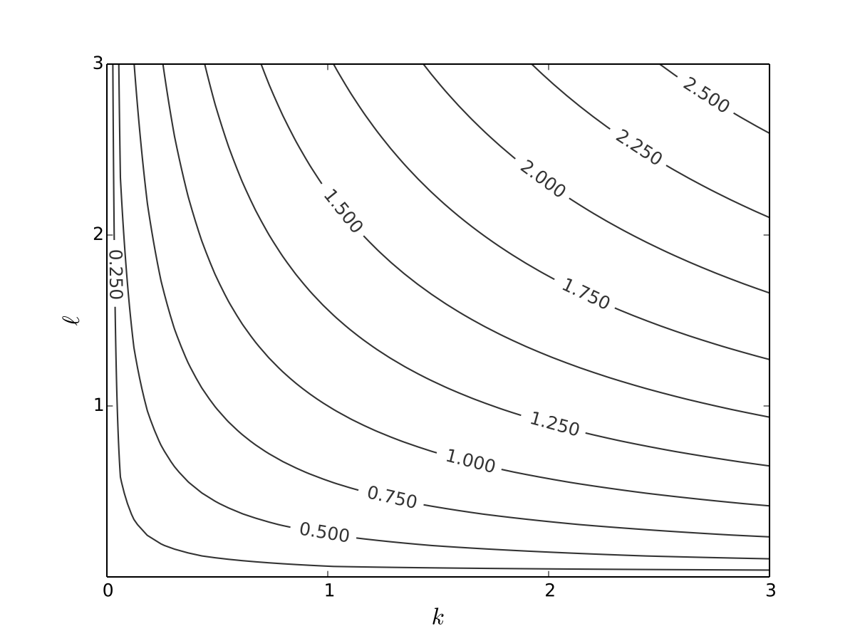
Fig. 10 Production function with \(\alpha=0.4\), \(\beta=0.5\)

Example: log-utility

Let \(u(x_1,x_2)\) be “utility” gained from \(x_1\) units of good 1 and \(x_2\) units of good 2

We take

\[ u(x_1, x_2) = \alpha \log(x_1) + \beta \log(x_2) \]

where

• \(\alpha\) and \(\beta\) are parameters

• we assume \(\alpha>0, \, \beta > 0\)

• The log functions mean “diminishing returns” in each good

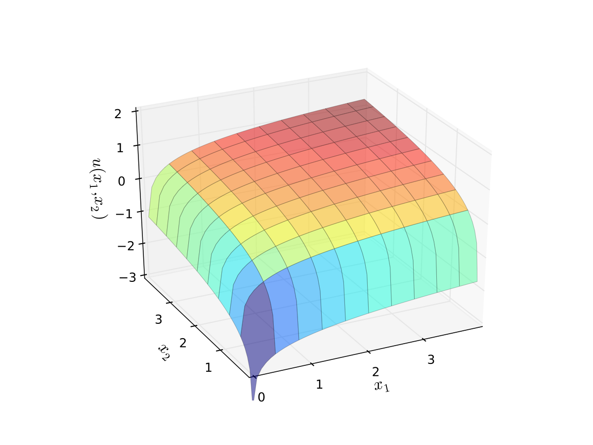
Fig. 11 Log utility with \(\alpha=0.4\), \(\beta=0.5\)

Let’s look at the contour lines

For utility functions, contour lines called indifference curves

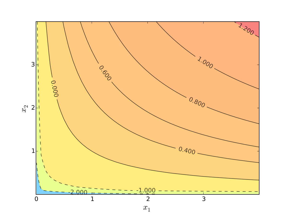
Fig. 12 Indifference curves of log utility with \(\alpha=0.4\), \(\beta=0.5\)

Example: quasi-linear utility

\[ u(x_1, x_2) = x_1 + \log(x_2) \]

• Called quasi-linear because linear in good 1

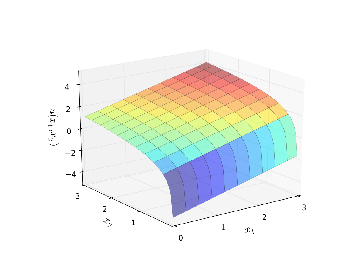
Fig. 13 Quasi-linear utility

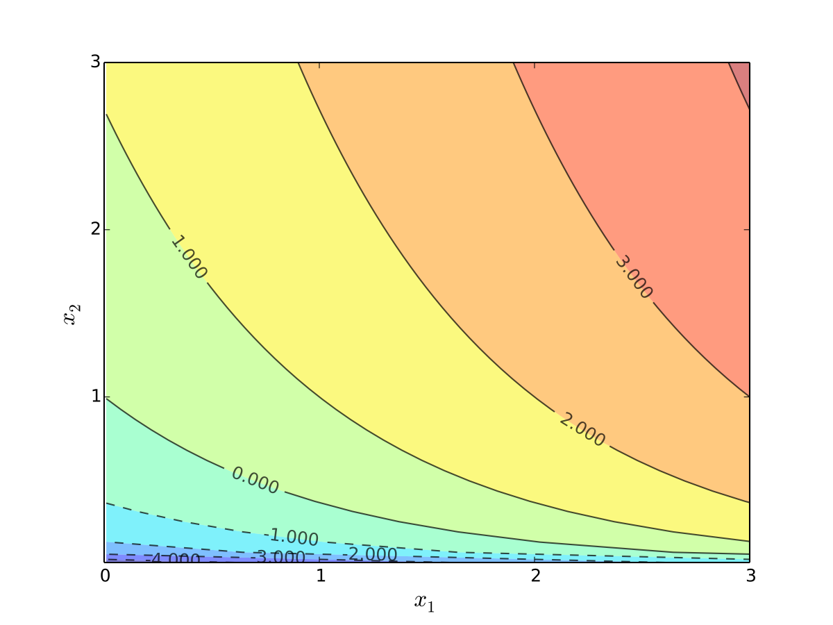
Fig. 14 Indifference curves of quasi-linear utility

Example: quadratic utility

\[ u(x_1, x_2) = - (x_1 - b_1)^2 - (x_2 - b_2)^2 \]

Here

• \(b_1\) is a “satiation” or “bliss” point for \(x_1\)

• \(b_2\) is a “satiation” or “bliss” point for \(x_2\)

Dissatisfaction increases with deviations from the bliss points

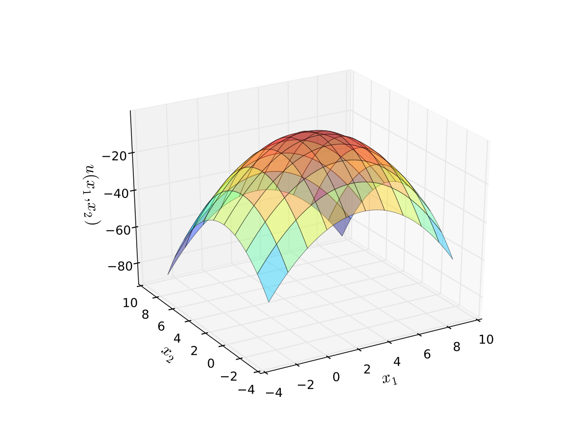
Fig. 15 Quadratic utility with \(b_1 = 3\) and \(b_2 = 2\)

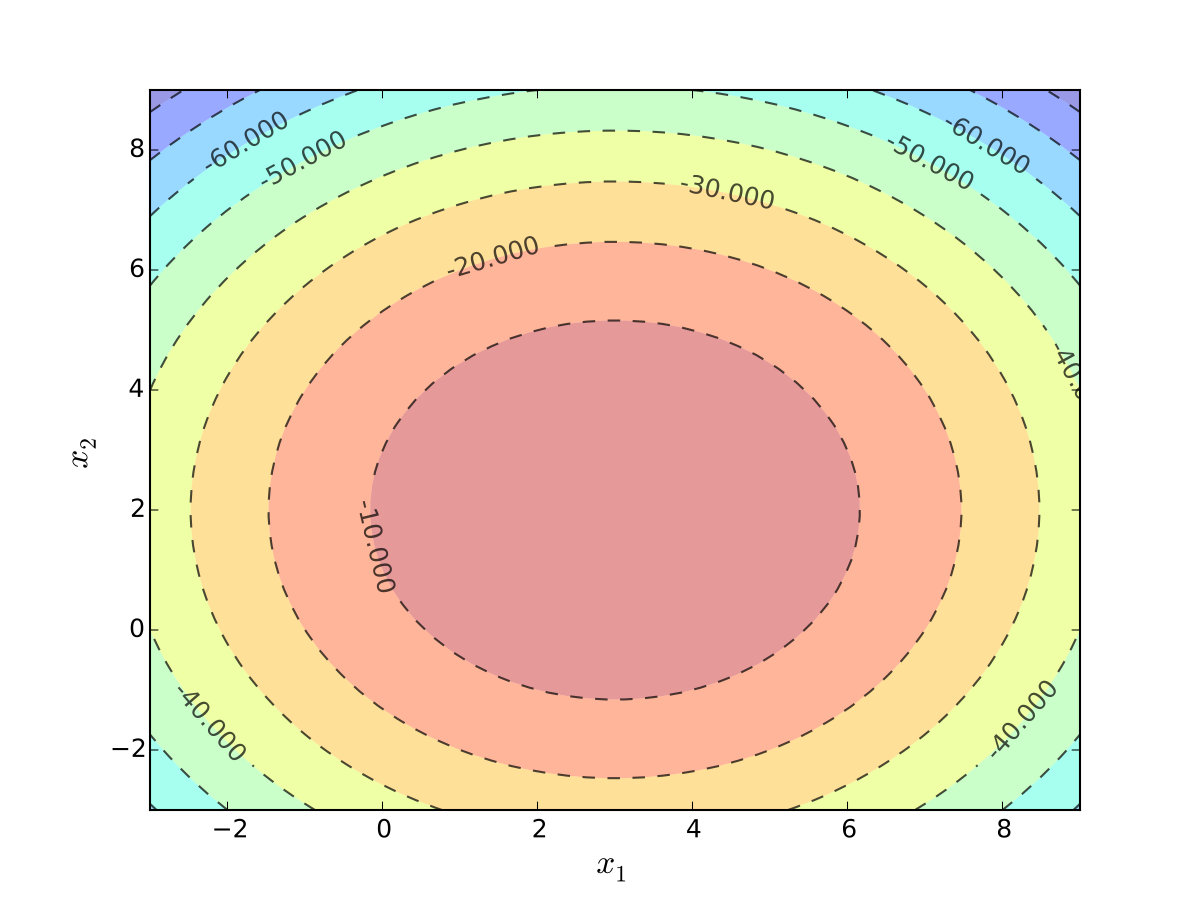
Fig. 16 Indifference curves quadratic utility with \(b_1 = 3\) and \(b_2 = 2\)

Bivariate Optimization

Consider \(f \colon I \to \mathbb{R}\) where \(I \subset \mathbb{R}^2\)

The set \(\mathbb{R}^2\) is all \((x_1, x_2)\) pairs

Definition

A point \((x_1^*, x_2^*) \in I\) is called a maximizer of \(f\) on \(I\) if

\[ f(x_1^*, x_2^*) \geq f(x_1, x_2) \quad \text{for all} \quad (x_1, x_2) \in I \]

Definition

A point \((x_1^*, x_2^*) \in I\) is called a minimizer of \(f\) on \(I\) if

\[ f(x_1^*, x_2^*) \leq f(x_1, x_2) \quad \text{for all} \quad (x_1, x_2) \in I \]

When they exist, the partial derivatives at \((x_1, x_2) \in I\) are

\[\begin{split} f_1(x_1, x_2) = \frac{\partial}{\partial x_1} f(x_1, x_2) \\ f_2(x_1, x_2) = \frac{\partial}{\partial x_2} f(x_1, x_2) \end{split}\]

Example

When \(f(k, \ell) = k^\alpha \ell^\beta\),

\[ f_1(k, \ell) = \frac{\partial}{\partial k} f(k, \ell) = \frac{\partial}{\partial k} k^\alpha \ell^\beta = \alpha k^{\alpha-1} \ell^\beta \]

Definition

An interior point \((x_1, x_2) \in I\) is called stationary for \(f\) if

\[ f_1(x_1, x_2) = f_2(x_1, x_2) = 0 \]

Fact

Let \(f \colon I \to \mathbb{R}\) be a continuously differentiable function. If \((x_1^*, x_2^*)\) is either

• an interior maximizer of \(f\) on \(I\), or

• an interior minimizer of \(f\) on \(I\),

then \((x_1^*, x_2^*)\) is a stationary point of \(f\)

Usage, for maximization:

1. Compute partials

2. Set partials to zero to find \(S =\) all stationary points

3. Evaluate candidates in \(S\) and boundary of \(I\)

4. Select point \((x^*_1, x_2^*)\) yielding highest value

Example

\[ f(x_1, x_2) = x_1^2 + 4 x_2^2 \rightarrow \min \quad \mathrm{s.t.} \quad x_1 + x_2 \leq 1 \]

Setting

\[ f_1(x_1, x_2) = 2 x_1 = 0 \quad \text{and} \quad f_2(x_1, x_2) = 8 x_2 = 0 \]

gives the unique stationary point \((0, 0)\), at which \(f(0, 0) = 0\)

On the boundary we have \(x_1 + x_2 = 1\), so

\[ f(x_1, x_2) = f(x_1, 1 - x_1) = x_1^2 + 4 (1 - x_1)^2 \]

Exercise: Show right hand side \(> 0\) for any \(x_1\)

Hence minimizer is \((x_1^*, x_2^*) = (0, 0)\)

Nasty secrets

Solving for \((x_1, x_2)\) such that \(f_1(x_1, x_2) = 0\) and \(f_2(x_1, x_2) = 0\) can be hard

• System of nonlinear equations

• Might have no analytical solution

• Set of solutions can be a continuum

Example

(Don’t) try to find all stationary points of

\[ f(x_1, x_2) = \frac{\cos(x_1^2 + x_2^2) + x_1^2 + x_1}{2 + p(-x_1^2) + \sin^2(x_2)} \]

Also:

• Boundary is often a continuum, not just two points

• Things get even harder in higher dimensions

On the other hand:

• Most classroom examples are chosen to avoid these problems

• Life is still pretty easy if we have concavity / convexity

• Clever tricks have been found for certain kinds of problems

Second Order Partials

Let \(f \colon I \to \mathbb{R}\) and, when they exist, denote

\[ f_{11}(x_1, x_2) = \frac{\partial^2}{\partial x_1^2} f(x_1, x_2) \]

\[ f_{12}(x_1, x_2) = \frac{\partial^2}{\partial x_1 \partial x_2} f(x_1, x_2) \]

\[ f_{21}(x_1, x_2) = \frac{\partial^2}{\partial x_2 \partial x_1} f(x_1, x_2) \]

\[ f_{22}(x_1, x_2) = \frac{\partial^2}{\partial x_2^2} f(x_1, x_2) \]

Example: Cobb-Douglas technology with linear costs

If \(\pi(k, \ell) = p k^{\alpha} \ell^{\beta} - w \ell - r k\) then

\[ \pi_{11}(k, \ell) = p \alpha(\alpha-1) k^{\alpha-2} \ell^{\beta} \]

\[ \pi_{12}(k, \ell) = p \alpha\beta k^{\alpha-1} \ell^{\beta-1} \]

\[ \pi_{21}(k, \ell) = p \alpha\beta k^{\alpha-1} \ell^{\beta-1} \]

\[ \pi_{22}(k, \ell) = p \beta(\beta-1) k^{\alpha} \ell^{\beta-2} \]

Fact

If \(f \colon I \to \mathbb{R}\) is twice continuously differentiable at \((x_1, x_2)\), then

\[ f_{12}(x_1, x_2) = f_{21}(x_1, x_2) \]

Exercise: Confirm the results in the exercise above.

Shape conditions in 2D

Let \(I\) be an “open” set (only interior points – formalities next week)

Let \(f \colon I \to \mathbb{R}\) be twice continuously differentiable

The function \(f\) is strictly concave on \(I\) if, for any \((x_1, x_2) \in I\)

1. \(f_{11}(x_1, x_2) < 0\)

2. \(f_{11}(x_1, x_2) \, f_{22}(x_1, x_2) > f_{12}(x_1, x_2)^2\)

The function \(f\) is strictly convex on \(I\) if, for any \((x_1, x_2) \in I\)

1. \(f_{11}(x_1, x_2) > 0\)

2. \(f_{11}(x_1, x_2) \, f_{22}(x_1, x_2) > f_{12}(x_1, x_2)^2\)

When is stationarity sufficient?

Fact

If \(f\) is differentiable and strictly concave on \(I\), then any stationary point of \(f\) is also a unique maximizer of \(f\) on \(I\)

Fact

If \(f\) is differentiable and strictly convex on \(I\), then any stationary point of \(f\) is also a unique minimizer of \(f\) on \(I\)

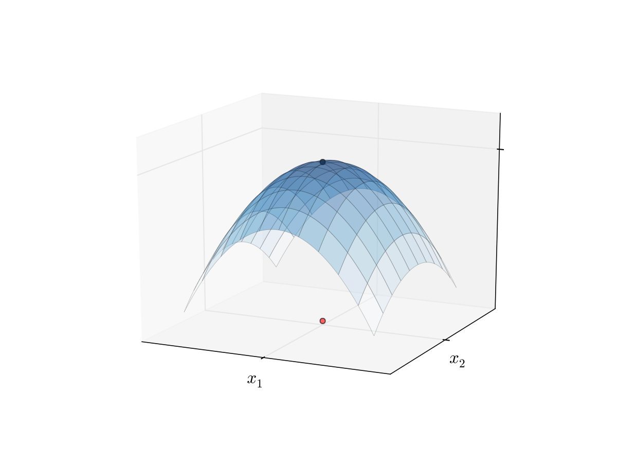
Fig. 17 Maximizer of a concave function

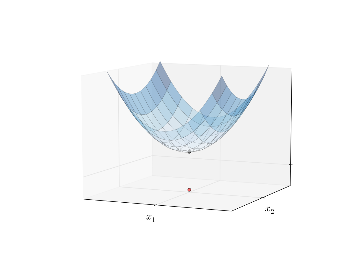
Fig. 18 Minimizer of a convex function

Example: unconstrained maximization of quadratic utility

\[ u(x_1, x_2) = - (x_1 - b_1)^2 - (x_2 - b_2)^2 \rightarrow \max_{x_1, x_2} \]

Intuitively the solution is \(x_1^*=b_1\) and \(x_2^*=b_2\)

Analysis above leads to the same conclusion

First let’s check first order conditions (F.O.C.)

\[ \frac{\partial}{\partial x_1} u(x_1, x_2) = -2 (x_1 - b_1) = 0 \quad \implies \quad x_1 = b_1 \]

\[ \frac{\partial}{\partial x_2} u(x_1, x_2) = -2 (x_2 - b_2) = 0 \quad \implies \quad x_2 = b_2 \]

How about (strict) concavity?

Sufficient condition is

1. \(u_{11}(x_1, x_2) < 0\)

2. \(u_{11}(x_1, x_2)u_{22}(x_1, x_2) > u_{12}(x_1, x_2)^2\)

We have

• \(u_{11}(x_1, x_2) = -2\)

• \(u_{11}(x_1, x_2)u_{22}(x_1, x_2) = 4 > 0 = u_{12}(x_1, x_2)^2\)

Example: Profit maximization with two inputs

\[ \pi(k, \ell) = p k^{\alpha} \ell^{\beta} - w \ell - r k \rightarrow \max_{k, \ell} \]

where \( \alpha, \beta, p, w\) are all positive and \(\alpha + \beta < 1\)

Derivatives:

• \(\pi_1(k, \ell) = p \alpha k^{\alpha-1} \ell^{\beta} - r\)

• \(\pi_2(k, \ell) = p \beta k^{\alpha} \ell^{\beta-1} - w\)

• \(\pi_{11}(k, \ell) = p \alpha(\alpha-1) k^{\alpha-2} \ell^{\beta}\)

• \(\pi_{22}(k, \ell) = p \beta(\beta-1) k^{\alpha} \ell^{\beta-2}\)

• \(\pi_{12}(k, \ell) = p \alpha \beta k^{\alpha-1} \ell^{\beta-1}\)

First order conditions: set

\[\begin{split} \pi_1(k, \ell) = 0 \\ \pi_2(k, \ell) = 0 \end{split}\]

and solve simultaneously for \(k, \ell\) to get

\[\begin{split} k^* = \left[ p (\alpha/r)^{1 - \beta} (\beta/w)^{\beta} \right]^{1 / (1 - \alpha - \beta)} \\ \ell^* = \left[ p (\beta/w)^{1 - \alpha} (\alpha/r)^{\alpha} \right]^{1 / (1 - \alpha - \beta)} \end{split}\]

Exercise: Verify

Now we check second order conditions, hoping for strict concavity

What we need: for any \(k, \ell > 0\)

1. \(\pi_{11}(k, \ell) < 0\)

2. \(\pi_{11}(k, \ell) \, \pi_{22}(k, \ell) > \pi_{12}(k, \ell)^2\)

Exercise: Show both inequalities satisfied when \(\alpha + \beta < 1\)

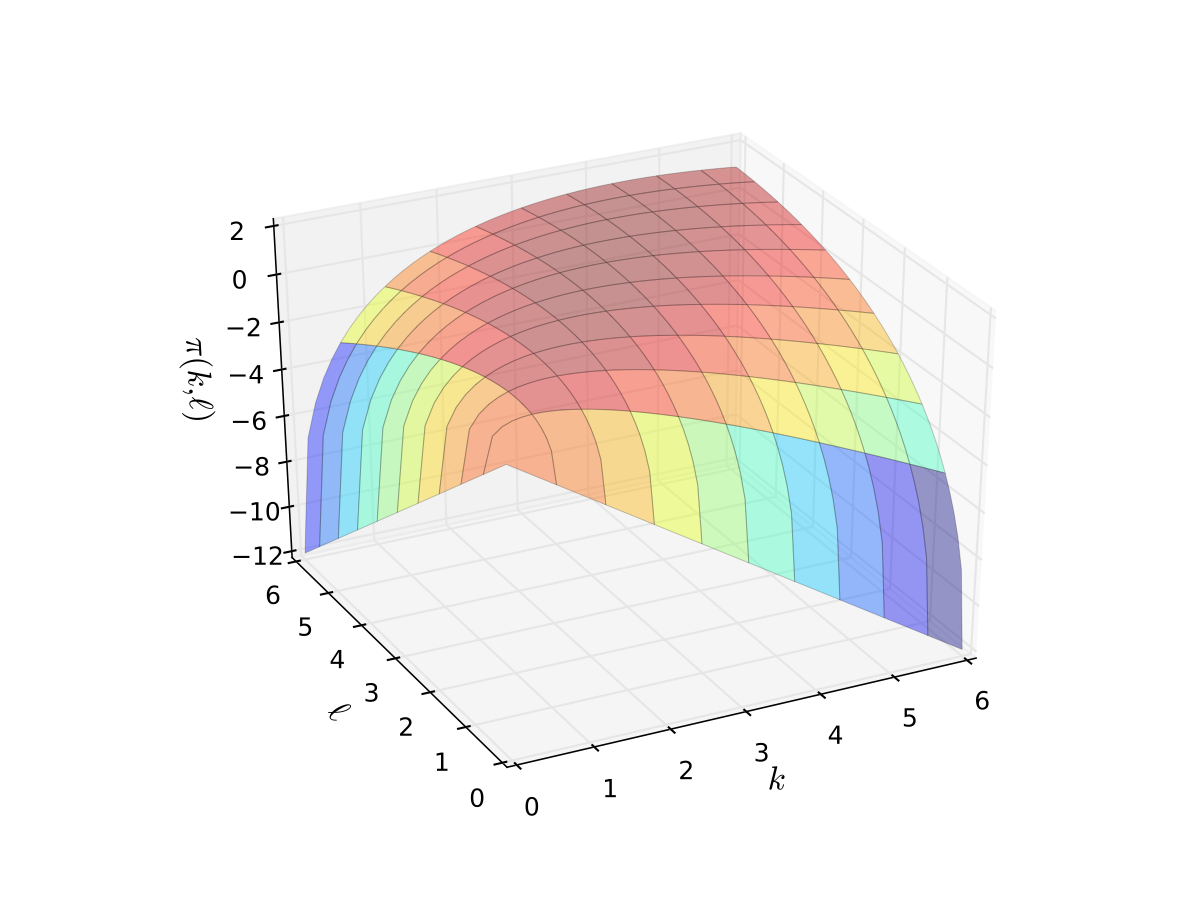
Fig. 19 Profit function when \(p=5\), \(r=w=2\), \(\alpha=0.4\), \(\beta=0.5\)

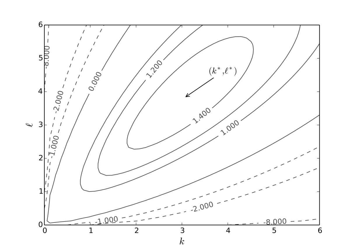
Fig. 20 Optimal choice, \(p=5\), \(r=w=2\), \(\alpha=0.4\), \(\beta=0.5\)