Fundamentals of optimization

ECON2125/6012 Lecture 6 Fedor Iskhakov

Announcements & Reminders

• Test 1 results and discussion

• Test 2 due date extended to Sept 6th (23:59)

Plan for this lecture

1. Open and closed sets (review)

2. Continuity of functions

3. Suprema and infima

4. Existence of optima

5. Uniqueness of optima

Supplementary reading:

• Simon & Blume: 12.2, 12.3, 12.4, 12.5, 13.4, 29.2, 30.1

• Sundaram: 1.2.6, 1.2.7, 1.2.8, 1.2.9, 1.2.10, 1.4.1, section 3

Sequences and limits in \(\mathbb{R}^K\)

Definition: sequence

A sequence \(\{{\bf x}_n\}\) in \(\mathbb{R}^K\) is a function from \(\mathbb{N}\) to \(\mathbb{R}^K\)

Definition: Euclidean norm

The (Euclidean) norm of \({\bf x} \in \mathbb{R}^N\) is defined as

\[ % \| {\bf x} \| := \sqrt{{\bf x}' {\bf x} } = \left( \sum_{n=1}^N x_n^2 \right)^{1/2} % \]

Interpretation:

• \(\| {\bf x} \|\) represents the length of \({\bf x}\)

• \(\| {\bf x} - {\bf y} \|\) represents distance between \({\bf x}\) and \({\bf y}\)

When \(K=1\), the norm \(\| \cdot \|\) reduces to \(|\cdot|\)

Definition

A set \(A \subset \mathbb{R}^K\) called bounded if

\[ % \exists \, M \in \mathbb{R} \; \mathrm{such\;that} \; \|{\bf x}\| \leq M, \quad \forall \; {\bf x} \in A % \]

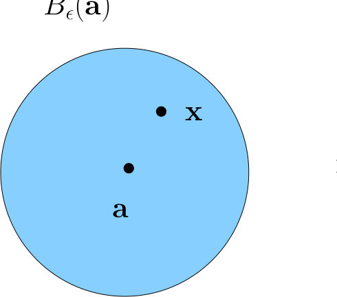
Definition

For \(\epsilon > 0\), the \(\epsilon\)-ball \(B_{\epsilon}({\bf a})\) around \({\bf a} \in \mathbb{R}^K\) is all \({\bf x} \in \mathbb{R}^K\) such that \(\|{\bf a} - {\bf x}\| < \epsilon\)

Fact

If \({\bf x}\) is in every \(\epsilon\)-ball around \({\bf a}\) then \({\bf x}={\bf a}\)

Fact

If \({\bf a} \ne {\bf b}\), then \(\exists \, \epsilon > 0\) such that \(B_\epsilon({\bf a}) \cap B_\epsilon({\bf b}) = \emptyset\)

Definition

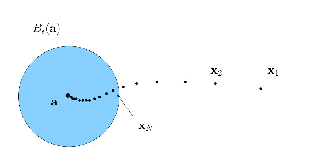
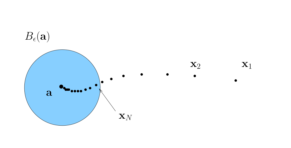
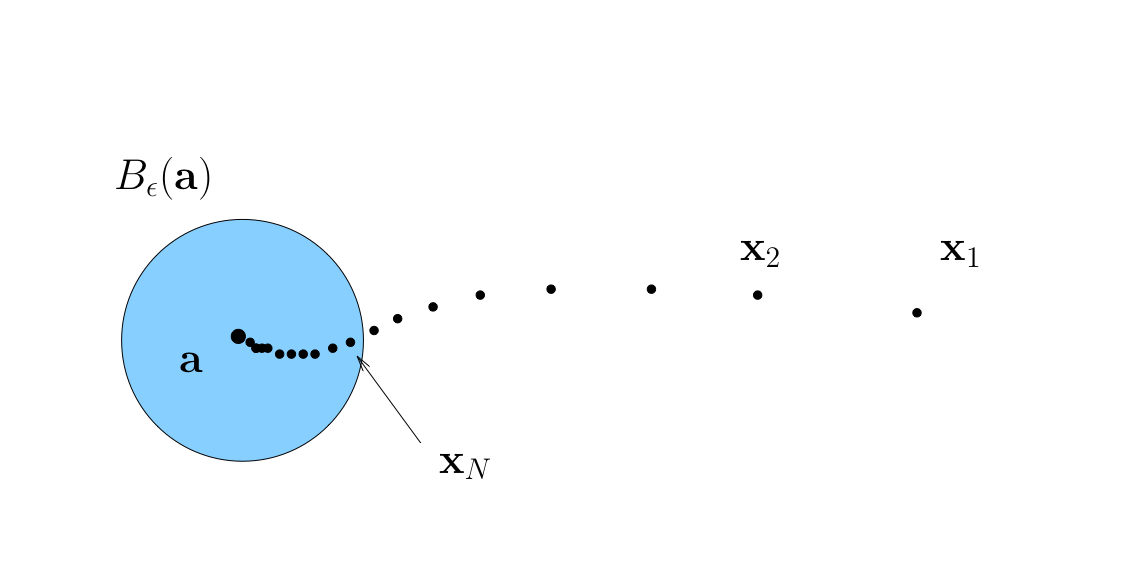
Sequence \(\{{\bf x}_n\}\) is said to converge to \({\bf a} \in \mathbb{R}^K\) if

\[ % \forall \epsilon > 0, \; \exists \, N \in \mathbb{N} \; \text{ such that } n \geq N \implies {\bf x}_n \in B_{\epsilon}({\bf a}) % \]

We say: “\(\{{\bf x}_n\}\) is eventually in any \(\epsilon\)-neighborhood of \({\bf a}\)”

In this case \({\bf a}\) is called the limit of the sequence, and we write

\[ % {\bf x}_n \to {\bf a} \; \text{ as } \; n \to \infty \quad \text{or} \quad \lim_{n \to \infty} {\bf x}_n = {\bf a} % \]

Definition

We call \(\{ {\bf x}_n \}\) convergent if it converges to some limit in \(\mathbb{R}^K\)

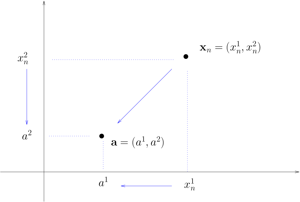
Fact

A sequence \(\{{\bf x}_n\}\) in \(\mathbb{R}^K\) converges to \({\bf a} \in \mathbb{R}^K\) if and only if each component sequence converges in \(\mathbb{R}\)

That is,

\[\begin{split} % \begin{pmatrix} x^1_n \\ \vdots \\ x^K_n \end{pmatrix} \to \begin{pmatrix} a^1 \\ \vdots \\ a^K \end{pmatrix} \quad \text{in } \mathbb{R}^K \quad \iff \quad \begin{array}{cc} x^1_n \to a^1 & \quad \text{in } \mathbb{R} \\ \vdots & \\ x^K_n \to a^K & \quad \text{in } \mathbb{R} \end{array} % \end{split}\]

\[ % {\bf x}_n \to {\bf a} \; \text{ in } \mathbb{R}^K % \quad \iff\quad % {\bf e}_k' {\bf x}_n \to {\bf e}_k' {\bf a} \text{ in $\mathbb{R}$ for all } k % \]

Open and Closed Sets

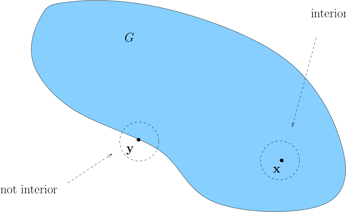
Let \(G \subset \mathbb{R}^K\)

Definition

We call \({\bf x} \in G\) interior to \(G\) if \(\exists \; \epsilon > 0\) with \(B_\epsilon({\bf x}) \subset G\)

Loosely speaking, interior means “not on the boundary”

Example

If \(G = (a, b)\) for some \(a < b\), then any \(x \in (a, b)\) is interior

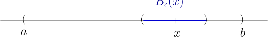
Proof

Fix any \(a < b\) and any \(x \in (a, b)\)

Let \(\epsilon := \min\{x - a, b - x\}\)

If \(y \in B_\epsilon(x)\) then \(y < b\) because

\[ % y = y + x - x \leq |y - x| + x < \epsilon + x \leq b - x + x = b % \]

Example

If \(G = [-1, 1]\), then \(1\) is not interior

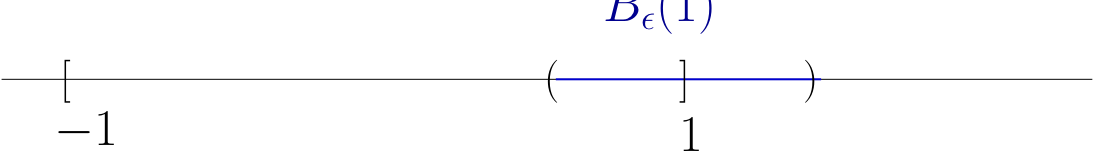
Intuitively, any \(\epsilon\)-ball centered on \(1\) will contain points \(> 1\)

More formally, pick any \(\epsilon > 0\) and consider \(B_\epsilon(1)\)

There exists a \(y \in B_\epsilon(1)\) such that \(y \notin [-1, 1]\)

For example, consider the point \(y := 1 + \epsilon/2\)

Exercise: Check this point: lies in \(B_\epsilon(1)\) but not in \([-1, 1]\)

Definition

A set \(G\subset \mathbb{R}^K\) is called open if all of its points are interior

Example

Open sets:

• any “open” interval \((a,b) \subset \mathbb{R}\), since we showed all points are interior

• any “open” ball \(B_\epsilon({\bf a}) = {\bf x} \in \mathbb{R}^K : \|{\bf x} - {\bf a} \| < \epsilon\)

• \(\mathbb{R}^K\) itself

Example

Sets that are not open

• \((a,b]\) because \(b\) is not interior

• \([a,b)\) because \(a\) is not interior

Closed Sets

Definition

A set \(F \subset \mathbb{R}^K\) is called closed if every convergent sequence in \(F\) converges to a point in \(F\)

Rephrased: If \(\{{\bf x}_n\} \subset F\) and \({\bf x}_n \to {\bf x}\) for some \({\bf x} \in \mathbb{R}^K\), then \({\bf x} \in F\)

Example

All of \(\mathbb{R}^K\) is closed because every sequence converging to a point in \(\mathbb{R}^K\) converges to a point in \(\mathbb{R}^K\)… right?

Example

If \((-1, 1) \subset \mathbb{R}\) is {\bf not} closed

Proof

True because

1. \(x_n := 1-1/n\) is a sequence in \((-1, 1)\) converging to \(1\),

2. and yet \(1 \notin (-1, 1)\)

Example

If \(F = [a, b] \subset \mathbb{R}\) then \(F\) is closed in \(\mathbb{R}\)

Proof

Take any sequence \(\{x_n\}\) such that

• \(x_n \in F\) for all \(n\)

• \(x_n \to x\) for some \(x \in \mathbb{R}\)

We claim that \(x \in F\)

Recall that (weak) inequalities are preserved under limits:

• \(x_n \leq b\) for all \(n\) and \(x_n \to x\), so \(x \leq b\)

• \(x_n \geq a\) for all \(n\) and \(x_n \to x\), so \(x \geq a\)

therefore \(x \in [a, b] =: F\)

Example

Any “hyperplane” of the form

\[ % H = \{ {\bf x} \in \mathbb{R}^K : {\bf x}' {\bf a} = c \} % \]

is closed

Proof

Fix \({\bf a} \in \mathbb{R}^K\) and \(c \in \mathbb{R}\) and let \(H\) be as above

Let \(\{{\bf x}_n\} \subset H\) with \({\bf x}_n \to {\bf x} \in \mathbb{R}^K\)

We claim that \({\bf x} \in H\)

Since \({\bf x}_n \in H\) and \({\bf x}_n \to {\bf x}\) we have

\[ % {\bf x}_n ' {\bf a} \to {\bf x}' {\bf a} \text{ in } \mathbb{R} \quad \text{and} \quad {\bf x}_n' {\bf a} = c \text{ for all } n % \]

\[ % \text{therefore } {\bf x}' {\bf a} = \lim_{n} {\bf x}_n' {\bf a} = \lim_n c = c % \]

\[ % \text{therefore } {\bf x} \in H % \]

Properties of Open and Closed Sets

Fact

\(G \subset \mathbb{R}^K\) is open \(\iff \; G^c\) is closed

Proof

\(\implies\)

First prove necessity

Pick any \(G\) and let \(F := G^c\)

Suppose to the contrary that \(G\) is open but \(F\) is not closed, so

\(\exists\) a sequence \(\{{\bf x}_n\} \subset F\) with limit \({\bf x} \notin F\)

Then \({\bf x} \in G\), and since \(G\) open, \(\exists \, \epsilon > 0\) such that \(B_\epsilon({\bf x}) \subset G\)

Since \({\bf x}_n \to {\bf x}\) we can choose an \(N \in \mathbb{N}\) with \({\bf x}_N \in B_\epsilon({\bf x})\)

This contradicts \({\bf x}_n \in F\) for all \(n\)

\(\Longleftarrow\)

Next prove sufficiency

Pick any closed \(F\) and let \(G := F^c\), need to prove that \(G\) is open

Suppose to the contrary that \(G\) is not open

Then exists some non-interior \({\bf x} \in G\), that is no \(\epsilon\)-ball around \(x\) lies entirely in \(G\)

Then it is possible to find a sequence \(\{{\bf x}_n\}\) which converges to \(x \in G\), but every element of which lies in the \(B_{1/n}({\bf x}) \cap F\)

This contradicts the fact that \(F\) is closed

Example

Any singleton \(\{ {\bf x} \} \subset \mathbb{R}^K\) is closed

Proof

Let’s prove this by showing that \(\{{\bf x}\}^c\) is open

Pick any \({\bf y} \in \{{\bf x}\}^c\)

We claim that \({\bf y}\) is interior to \(\{{\bf x}\}^c\)

Since \({\bf y} \in \{{\bf x}\}^c\) it must be that \({\bf y} \ne {\bf x}\)

Therefore, exists \(\epsilon > 0\) such that \(B_\epsilon({\bf y}) \cap B_\epsilon({\bf x}) = \emptyset\)

In particular, \({\bf x} \notin B_\epsilon({\bf y})\), and hence \(B_\epsilon({\bf y}) \subset \{{\bf x}\}^c\)

Therefore \({\bf y}\) is interior as claimed

Since \({\bf y}\) was arbitrary it follows that \(\{{\bf x}\}^c\) is open and \(\{{\bf x}\}\) is closed

Fact

1. Any union of open sets is open

2. Any intersection of closed sets is closed

Proof

Proof of first fact:

Let \(G := \cup_{\lambda \in \Lambda} G_\lambda\), where each \(G_\lambda\) is open

We claim that any given \({\bf x} \in G\) is interior to \(G\)

Pick any \({\bf x} \in G\)

By definition, \({\bf x} \in G_\lambda\) for some \(\lambda\)

Since \(G_\lambda\) is open, \(\exists \, \epsilon > 0\) such that \(B_\epsilon({\bf x}) \subset G_\lambda\)

But \(G_\lambda \subset G\), so \(B_\epsilon({\bf x}) \subset G\) also holds

In other words, \({\bf x}\) is interior to \(G\)

But be careful:

• An infinite intersection of open sets is not necessarily open

• An infinite union of closed sets is not necessarily closed

For example, if \(G_n := (-1/n, 1/n)\), then \(\cap_{n \in \mathbb{N}} G_n = \{0\} \)

To see this, suppose that \(x \in \cap_n G_n\)

Then

\[ % -1/n < x < 1/n, \quad \forall n \in \mathbb{N} % \]

Therefore \(x = 0\), and hence \(x \in \{0\}\)

On the other hand, if \(x \in \{0\}\) then \(x \in \cap_n G_n\)

Fact

If \(A\) is closed and bounded then every sequence in \(A\) has a subsequence which converges to a point of \(A\)

Take any sequence \(\{{\bf x}_n\}\) contained in \(A\)

Since \(A\) is bounded, \(\{{\bf x}_n\}\) is bounded

Therefore it has a convergent subsequence

Since the subsequence is also contained in \(A\), and \(A\) is closed, the limit must lie in \(A\).

Definition

Bounded and closed sets are called compact sets or compacts

Continuity

One of the most fundamental properties of functions

Related to existence of

• optima

• roots

• fixed points

• etc

as well as a variety of other useful concepts

Reminder on functions >>

Definition

A function \(f \colon A \rightarrow B\) from set \(A\) to set \(B\) is a rule that associates to each element of \(A\) a uniquely determined element of \(B\)

\(A\) is called the domain of \(f\) and \(B\) is called the codomain

Lower panel: functions have to map all elements in domain to a uniquely determined element in codomain.

Definition

The smallest possible codomain is called the range of \(f \colon A \to B\):

\[ % \mathrm{rng}(f) := \{ b \in B : f(a) = b \text{ for some } a \in A \} % \]

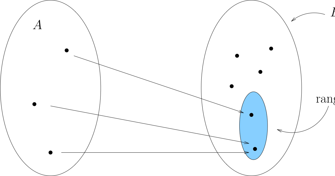
Definition

A function \(f \colon A \to B\) is called onto (or surjection) if every element of \(B\) is the image under \(f\) of at least one point in \(A\).

A function \(f \colon A \to B\) is called one-to-one (or injection) if distinct elements of \(A\) are always mapped into distinct elements of \(B\).

A function that is both one-to-one (injection) and onto (surjection) is called a bijection or one-to-one correspondence

Fact

If \(f \colon A \to B\) is one-to-one, then \(f \colon A \to \mathrm{rng}(f)\) is a bijection

Fact

If \(f \colon A \to B\) a bijection, then there exists a unique function \(\phi \colon B \to A\) such that

\[ % \phi(f(a)) = a, \quad \forall \; a \in A % \]

That function \(\phi\) is called the inverse of \(f\) and written \(f^{-1}\)

Bounded functions

Definition

A function \(F\) is called bounded if its range is a bounded set.

Fact

If \(F\) and \(G\) are bounded, then so are \(F+G\), \(F \cdot G\) and \(\alpha F\) for any finite \(\alpha\)

Proof

Proof for the case \(F + G\):

Let \(F\) and \(G\) be bounded functions

\(\exists\) \(M_F\) and \(M_G\) s.t. \(\| F({\bf x}) \| \leq M_F\) and \(\| G({\bf x}) \| \leq M_G\) for all \({\bf x}\)

Fix any \({\bf x}\) and let \(M := M_F + M_G\)

Applying the triangle inequality gives

\[ % \| (F + G)({\bf x}) \| := \| F({\bf x}) + G({\bf x}) \| \leq \| F({\bf x}) \| + \| G({\bf x}) \| \leq M % \]

Since \({\bf x}\) was arbitrary this bound holds for all \({\bf x}\)

Continuous functions

Definition

Let \(F \colon A \to \mathbb{R}^J\) where \(A\) is a subset of \(\mathbb{R}^K\). \(F\) is called continuous at \({\bf x} \in A\) if as \(n \to \infty\)

\[ % {\bf x}_n \to {\bf x} \quad \implies \quad F({\bf x}_n) \to F({\bf x}) % \]

Requires that

• \(F({\bf x}_n)\) converges for each choice of \({\bf x}_n \to {\bf x}\),

• The limit is always the same, and that limit is \(F({\bf x})\)

Definition

\(F\) is called continuous if it is continuous at every \({\bf x} \in A\)

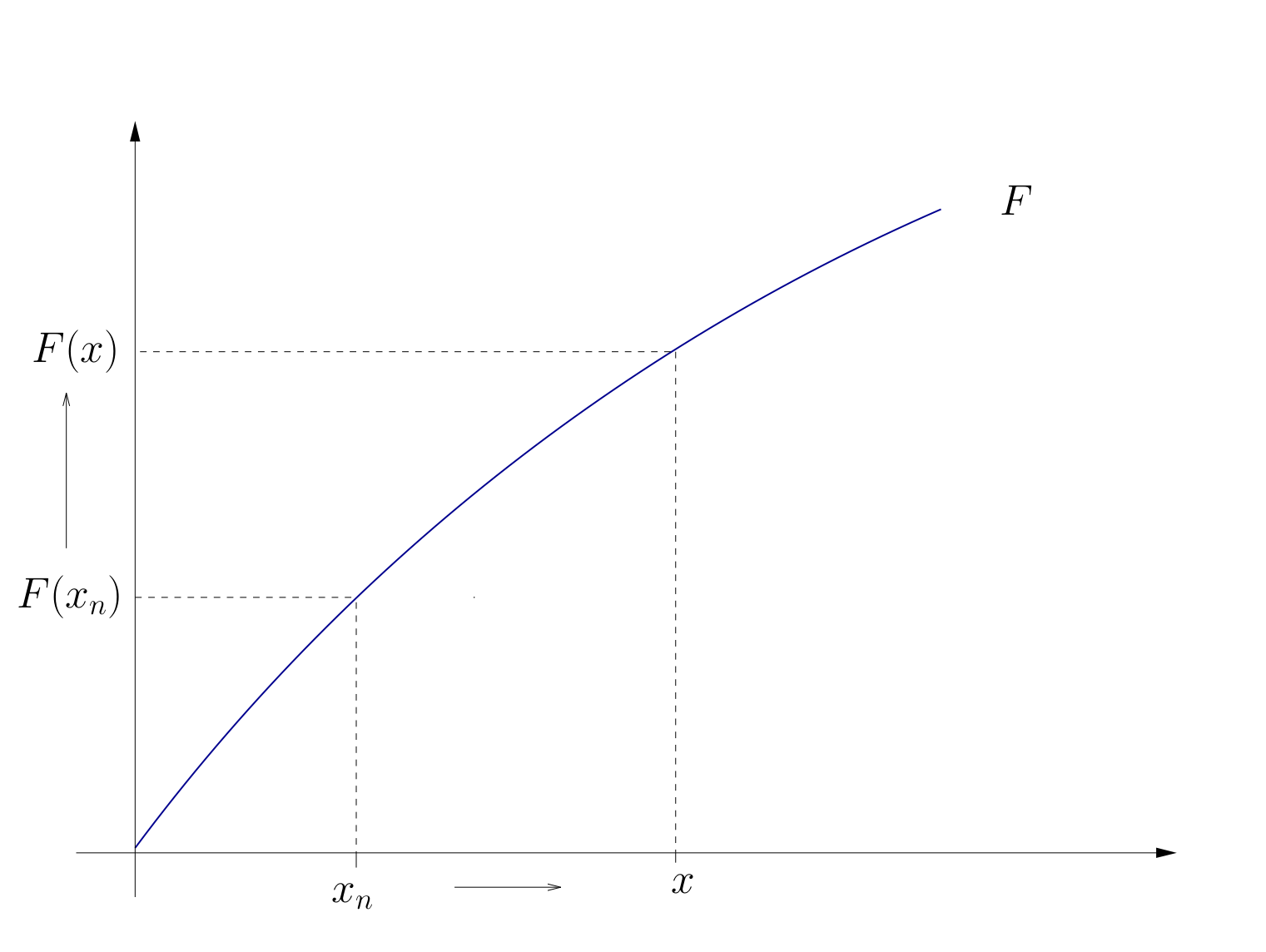
Fig. 73 Continuity

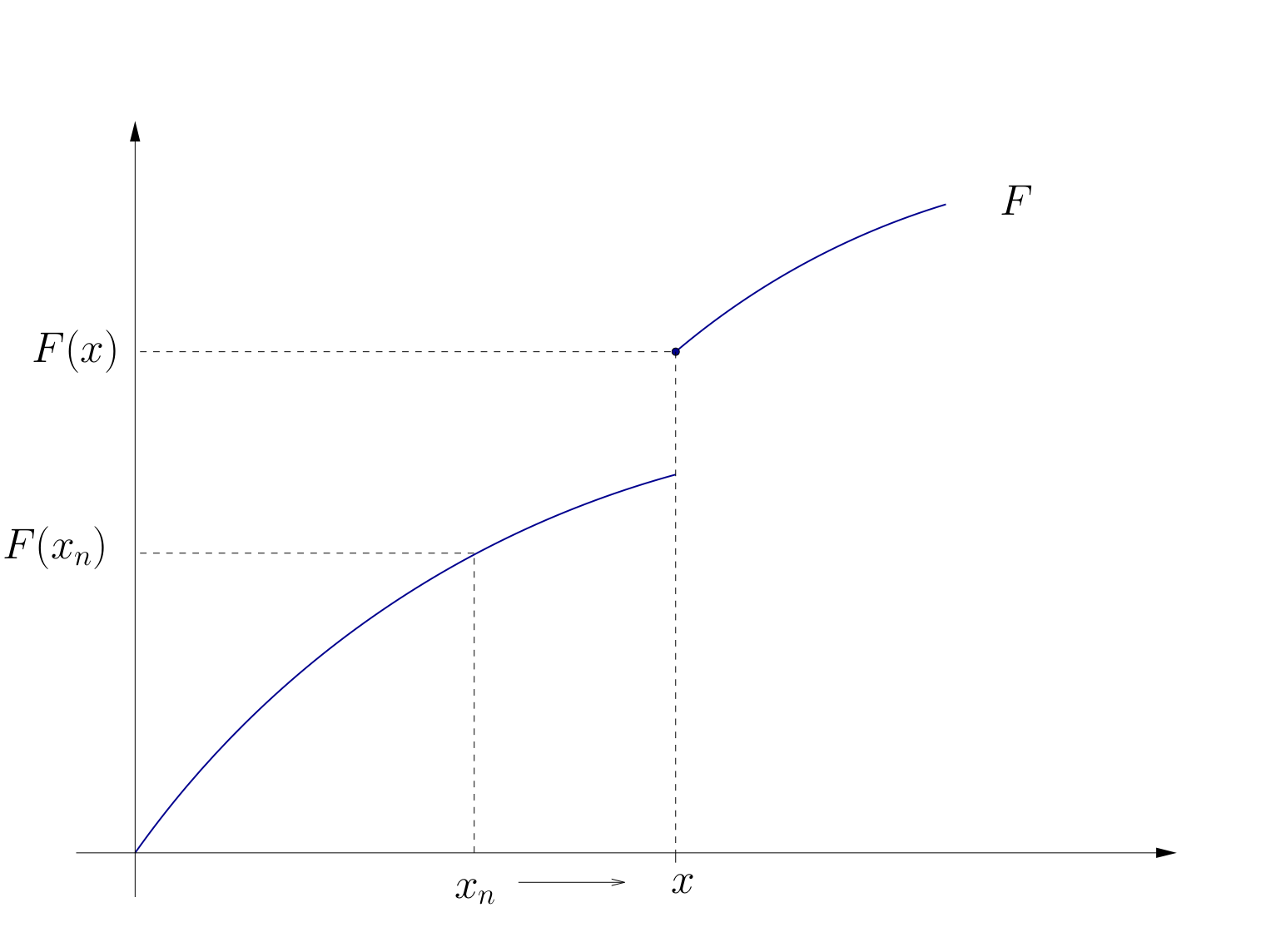
Fig. 74 Discontinuity at \(x\)

Example

Let \({\bf A}\) be an \(J \times K\) matrix and let \(F({\bf x}) = {\bf A} {\bf x}\)

The function \(F\) is continuous at every \({\bf x} \in \mathbb{R}^K\)

To see this take

• any \({\bf x} \in \mathbb{R}^K\)

• any \({\bf x}_n \to {\bf x}\)

By the definition of the matrix norm \(\| {\bf A} \|\), we have

\[ % \| {\bf A} {\bf x}_n - {\bf A} {\bf x} \| = \| {\bf A} ({\bf x}_n - {\bf x}) \| \leq \| {\bf A} \| \| {\bf x}_n - {\bf x} \| % \]

\[ % \text{therefore } {\bf x}_n \to {\bf x} \implies {\bf A} {\bf x}_n \to {\bf A} {\bf x} % \]

Exercise: Exactly what rules are we using here?

Fact

If \(f \colon \mathbb{R} \to \mathbb{R}\) is differentiable at \(x\), then \(f\) is continuous at \(x\)

\[ %\frac{f(x + h_n) - f(x)}{h_n} %= %\frac{f(x_n) - f(x)}{x_n - x} %% \]

Fact

Some functions known to be continuous on their domains:

• \(x \mapsto x^\alpha\)

• \(x \mapsto |x|\)

• \(x \mapsto \log(x)\)

• \(x \mapsto \exp(x)\)

• \(x \mapsto \sin(x)\)

• \(x \mapsto \cos(x)\)

Example

Discontinuous at zero: \(x \mapsto \mathbb{1}\{x > 0\}\).

Fact

Let \(F\) and \(G\) be functions and let \(\alpha \in \mathbb{R}\)

1. If \(F\) and \(G\) are continuous at \({\bf x}\) then so is \(F + G\), where

\[ % (F + G)({\bf x}) := F({\bf x}) + G({\bf x}) % \]

2. If \(F\) is continuous at \({\bf x}\) then so is \(\alpha F\), where

\[ % (\alpha F)({\bf x}) := \alpha F({\bf x}) % \]

3. If \(F\) and \(G\) are continuous at \({\bf x}\) and real valued then so is \(FG\), where

\[ % (FG)({\bf x}) := F({\bf x}) \cdot G({\bf x}) % \]

In the latter case, if in addition \(G({\bf x}) \ne 0\), then \(F/G\) is also continuous.

As a result, set of continuous functions is “closed” under elementary arithmetic operations

Example

The function \(F \colon \mathbb{R} \to \mathbb{R}\) defined by

\[ % F(x) = \frac{\exp(x) + \sin(x)}{2 + \cos(x)} + \frac{x^4}{2} - \frac{\cos^3(x)}{8!} % \]

is continuous

Proof

Just repeatedly apply the rules on the previous slide

Let’s just check that

\[ % \text{$F$ and $G$ continuous at ${\bf x}$} \implies \text{$F + G$ continuous at ${\bf x}$} % \]

Let \(F\) and \(G\) be continuous at \({\bf x}\)

Pick any \({\bf x}_n \to {\bf x}\)

We claim that \(F({\bf x}_n) + G({\bf x}_n) \to F({\bf x}) + G({\bf x})\)

By assumption, \(F({\bf x}_n) \to F({\bf x})\) and \(G({\bf x}_n) \to G({\bf x})\)

From this and the triangle inequality we get

\[ % \| F({\bf x}_n) + G({\bf x}_n) - (F({\bf x}) + G({\bf x})) \| \leq % \]

\[ % \leq \| F({\bf x}_n) - F({\bf x}) \| + \| G({\bf x}_n) - G({\bf x}) \| \to 0 % \]

End of review, new topic next >>>

Suprema and Infima (\(\mathrm{sup}\) + \(\mathrm{inf}\))

In the introductory lecture we have seen a few simple examples of optimization problems. Like in many introductory econ/finance cources we get well behaved, prepackaged problems.

Usually they

• have a solution

• the solution is unique and not hard to find

However, for the majority of problems such properties aren’t guaranteed

We need some idea of how to check these things

Consider the problem of finding the “maximum” or “minimum” of a function

A first issue is that such values might not be well defined

Recall that the set of maximizers/minimizers can be

• empty

• a singleton (contains one element)

• infinite (contains infinitely many elements)

Show code cell content Hide code cell content

from myst_nb import glue
import matplotlib.pyplot as plt
import numpy as np

def subplots():
    "Custom subplots with axes through the origin"
    fig, ax = plt.subplots()
    # Set the axes through the origin
    for spine in ['left', 'bottom']:
        ax.spines[spine].set_position('zero')
    for spine in ['right', 'top']:
        ax.spines[spine].set_color('none')
    return fig, ax

xmin, xmax = 0, 1
xgrid1 = np.linspace(xmin, xmax, 100)
xgrid2 = np.linspace(xmax, 2, 10)

fig, ax = subplots()
ax.set_ylim(0, 1.1)
ax.set_xlim(-0.0, 2)
func_string = r'$f(x) = x^2$ if $x < 1$ else $f(x) = 0.5$'
ax.plot(xgrid1, xgrid1**2, 'b-', lw=3, alpha=0.6, label=func_string)
ax.plot(xgrid2, 0 * xgrid2 + 0.5, 'b-', lw=3, alpha=0.6)
#ax.legend(frameon=False, loc='lower right', fontsize=16)
glue("fig_none", fig, display=False)

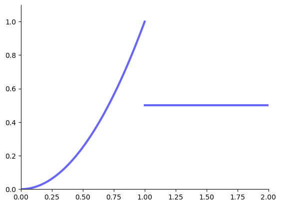
Example: no maximizers

The following function has no maximizers on \([0, 2]\)

\[\begin{split} f(x) = \begin{cases} x^2 & \text{ if } x < 1 \\ 1/2 & \text{ otherwise} \end{cases} \end{split}\]

Fig. 75 No maximizer on \([0, 2]\)

This leads us to start with “suprema” and “infima”

• Always well defined

• Agree with max and min when the latter exist

Definition

Let \(A \subset \mathbb{R}\). A number \(u \in \mathbb{R}\) is called an upper bound of \(A\) if

\[ % a \leq u \quad \text{for all} \quad a \in A % \]

Example

If \(A = (0, 1)\) then 10 is an upper bound of \(A\)

\(\because \quad\) Every element of \((0, 1)\) is \(\leq 10\)

Example

If \(A = (0, 1)\) then 1 is an upper bound of \(A\)

\(\because \quad\) Every element of \((0, 1)\) is \(\leq 1\)

Example

If \(A = (0, 1)\) then \(0.5\) is not an upper bound of \(A\)

\(\because \quad\) \(\exists\, a = 0.6 \in (0, 1) = A\) and \(0.5 < 0.6\)

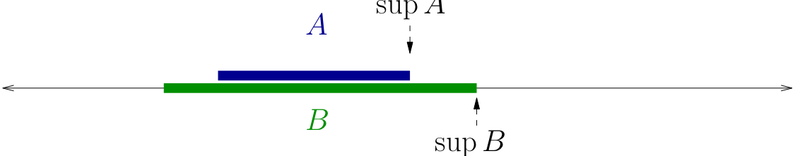
Let \(U(A) :=\) set of all upper bounds of \(A\)

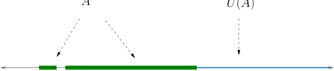
Examples

• If \(A = [0, 1]\), then \(U(A) = [1, \infty)\)

• If \(A = (0, 1)\), then \(U(A) = [1, \infty)\)

• If \(A = (0, 1) \cup (2, 3)\), then \(U(A) = [3, \infty)\)

• If \(A = \mathbb{N}\), then \(U(A) = \emptyset\)

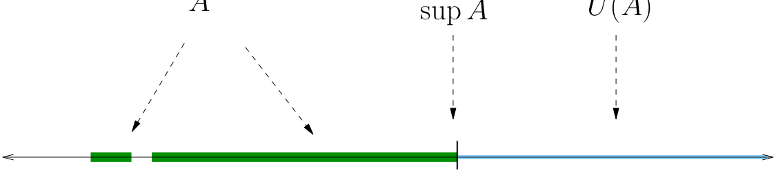
Definition

The least upper bound of \(A\) is called supremum of \(A\).

In other words, if \(s\) is a number satisfying

\[ % s \in U(A) \qquad \text{and} \qquad s \leq u, \; \forall \, u \in U(A) % \]

then \(s\) is the supremum of \(A\) and we write \(s = \sup A\)

Example

If \(A = (0, 1]\), then \(U(A) = [1, \infty)\), so \(\sup A = 1\)

Example

If \(A = (0, 1)\), then \(U(A) = [1, \infty)\), so \(\sup A = 1\)

Definition

A set \(A \subset \mathbb{R}\) is called bounded above if \(U(A)\) is not empty

Fact

If \(A\) is nonempty and bounded above then \(A\) has a supremum in \(\mathbb{R}\)

• Equivalent to the fact that all Cauchy sequences converge

• Same principle: \(\mathbb{R}\) has no “gaps” or “holes”

What if \(A\) is not bounded above, so that \(U(A) = \emptyset\)?

We follow the convention that \(\sup A := \infty\) in this case

Now the supremum of a nonempty subset of \(\mathbb{R}\) always exists

Note

Aside: Conventions for dealing with symbols “\(\infty\)’’ and ``\(-\infty\)”

If \(a \in \mathbb{R}\), then

• \(a + \infty = \infty\)

• \(a - \infty = -\infty\)

• \(a \times \infty = \infty\) if \(a \ne 0\), \(0 \times \infty = 0\)

• \(-\infty < a < \infty\)

• \(\infty + \infty = \infty\)

• \(-\infty - \infty = -\infty\)

But \(\infty - \infty\) is not defined

Fact

If \(A \subset B\), then \(\sup A \leq \sup B\)

Proof

Let \(A \subset B\)

If \(\sup B = \infty\) then the claim is trivial so suppose \(\bar b = \sup B < \infty\)

By definition, \(\bar b \in U(B)\), so \(b \leq \bar b\) for all \(b \in B\)

Since each \(a \in A\) is also in \(B\), we then have \(a \leq \bar b\) for all \(a \in A \)

It follows that \(\bar b \in U(A)\)

Hence \(\sup A \leq \bar b\)

Fact

Let \(A\) be any set bounded from above and let \(s := \sup A\). There exists a sequence \(\{x_n\}\) in \(A\) with \(x_n \to s\).

Proof

Note that

\[ % \forall \, n \in \mathbb{N}, \;\; \exists \, x_n \in A \; \text{ such that } \; x_n > s - \frac{1}{n} % \]

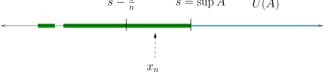
(Otherwise \(s\) is not a sup, because \(s-\frac{1}{n}\) is a smaller upper bound)

The sequence \(\{x_n\}\) lies in \(A\) and converges to \(s\)

Definition

A lower bound of \(A \subset \mathbb{R}\) is any \(\ell \in \mathbb{R}\) with \(\ell \leq a\) for all \(a \in A\)

Definition

If \(i \in \mathbb{R}\) is an lower bound for \(A\) with \(i \geq \ell\) for every lower bound \(\ell\) of \(A\), then \(i\) is called the infimum of \(A\)

Infimum is written as \(i = \inf A\)

Example

• If \(A = [0, 1]\), then \(\inf A = 0\)

• If \(A = (0, 1)\), then \(\inf A = 0\)

Fact

Every nonempty subset of \(\mathbb{R}\) bounded from below has an infimum

If \(A\) is unbounded below then we set \(\inf A = -\infty\)

Maxima and Minima of Sets

In optimization we’re mainly interested in maximizing and minimizing functions

\[ % \max_{{\bf x} \in A} f({\bf x}) % \]

As we’ll see, the problem is the same as finding the largest number in the range of \(f\)

That is, the largest number in the set

\[ f(A) := \{ f({\bf x}) \colon {\bf x } \in A\} \]

Definition

We call \(a^*\) the maximum of \(A \subset \mathbb{R}\) and write \(a^* = \max A\) if

\[ % a^* \in A \qquad \text{and} \qquad a \leq a^* \text{ for all } a \in A % \]

Example

If \(A = [0, 1]\) then \(\max A = 1\)

Definition

We call \(a^*\) the minimum of \(A \subset \mathbb{R}\) and write \(a^* = \min A\) if

\[ % a^* \in A \qquad \text{and} \qquad a^* \leq a \text{ for all } a \in A % \]

Example

If \(A = [0, 1]\) then \(\min A = 0\)

Fact

If \(A \subset \mathbb{R}\) is finite then \(\max A\) and \(\min A\) always exist

Example

• \(\max\{2, 4, 6, 8\} = 8\)

• \(\min\{2, 4, 6, 8\} = 2\)

Fact

For infinite subsets of \(\mathbb{R}\), max and min may not exist!

Example

\(\max \mathbb{N}\) does not exist

Proof

Suppose to the contrary that \(n^* = \max \mathbb{N}\)

By the definition of the maximum, \(n^* \in \mathbb{N}\)

Now consider

\[ % n^{**} := n^* + 1 % \]

Clearly

\[ % n^{**} \in \mathbb{N} \quad \text{and} \quad n^{**} > n^* % \]

This contradicts the definition of \(n^*\)

Example

\(\max (0, 1)\) does not exist

Proof

Suppose to the contrary that \(a^* = \max (0, 1)\)

By the definition of the maximum, \(a^* \in (0, 1)\)

Hence \(a^* < 1\)

Now consider

\[ % a^{**} := (1 + a^*)/2 % \]

Clearly

\[ % a^{**} \in (0, 1) \text{ and } a^{**} > a^* % \]

Contradicts hypothesis that \(a^*\) is the maximum

Relationship between max/min and sup/inf

When max and min exist they agree with sup and inf

Fact

Let \(A\) be any subset of \(\mathbb{R}\)

1. If \(\sup A \in A\), then \(\max A\) exists and \(\max A = \sup A\)

2. If \(\inf A \in A\), then \(\min A\) exists and \(\min A = \inf A\)

Proof

Proof of case 1: Let \(a^* := \sup A\) and suppose \(a^* \in A\)

We want to show that \(\max A = a^*\)

Since \(a^* \in A\), we need only show that \(a \leq a^*\) for all \(a \in A\)

This follows from \(a^* = \sup A\), which implies \(a^* \in U(A)\)

Fact

If \(F \subset \mathbb{R}\) is a closed and bounded, then \(\max F\) and \(\min F\) both exist

Proof

Proof for the max case:

Since \(F\) is bounded,

• \(\sup F\) exists

• \(\exists\) a sequence \(\{x_n\} \subset F\) with \(x_n \to \sup F\)

Since \(F\) is closed, this implies that \(\sup F \in F\)

Hence \(\max F\) exists and \(\max F = \sup F\)

Existence of optima for functions

Now we turn to suprema and infima, maxima and minima (extrema) for functions

This is not a new concept — it’s just about extrema of sets — but the sets are the range of functions

In particular

• The sup of a function \(f\) is just the sup of its range

• The max of a function \(f\) is just the max of its range

Througout we use the notation

\[ f(A) := \{ f({\bf x}) \colon {\bf x } \in A\} \]

Definition

Let \(f \colon A \to \mathbb{R}\), where \(A\) is any set

The supremum of \(f\) on \(A\) is defined as

\[ % \sup_{{\bf x} \in A} f({\bf x}) := \sup f(A) % \]

The infimum of \(f\) on \(A\) is defined as

\[ % \inf_{{\bf x} \in A} f({\bf x}) := \inf f(A) % \]

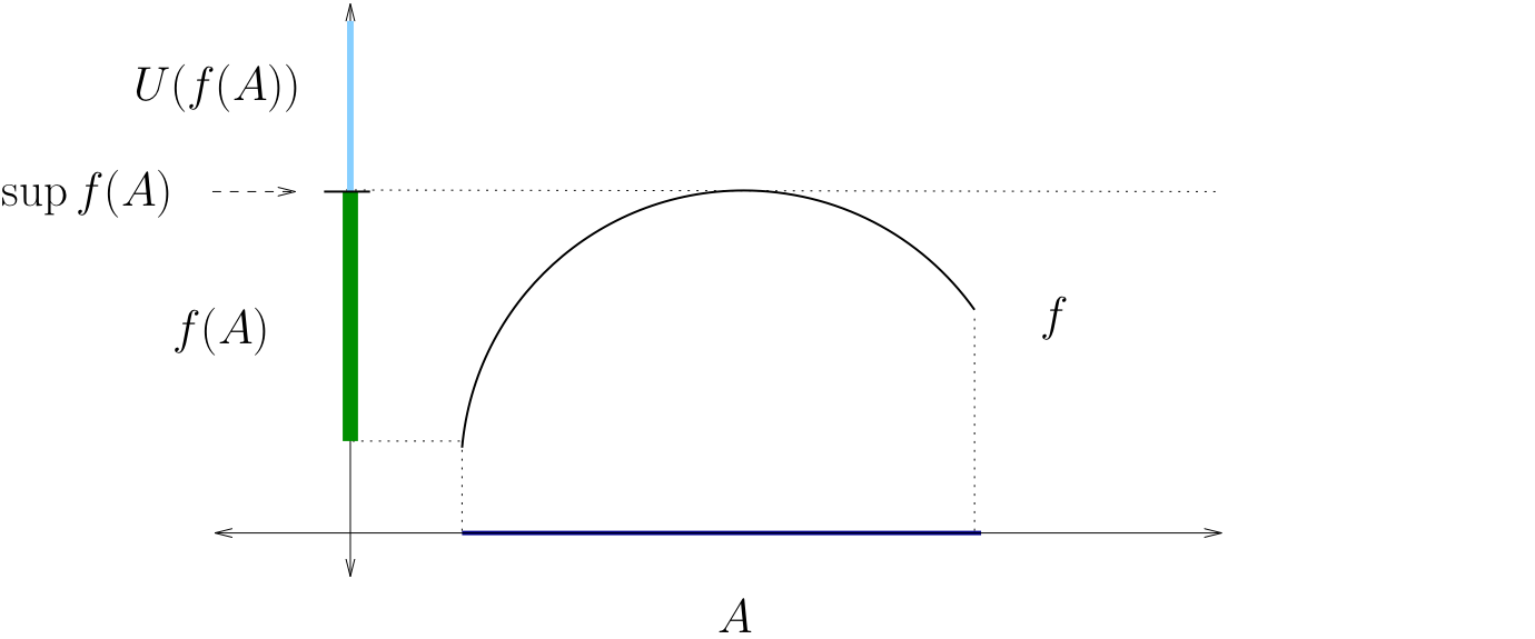
Fig. 76 The supremum of \(f\) on \(A\)

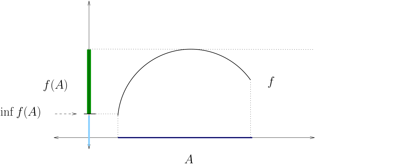
Fig. 77 The infimum of \(f\) on \(A\)

Definition

Let \(f \colon A \to \mathbb{R}\) where \(A\) is any set

The maximum of \(f\) on \(A\) is defined as

\[ % \max_{{\bf x} \in A} f({\bf x}) := \max f(A) % \]

The minimum of \(f\) on \(A\) is defined as

\[ % \min_{{\bf x} \in A} f({\bf x}) := \min f(A) % \]

Definition

A maximizer of \(f\) on \(A\) is a point \({\bf a}^* \in A\) such that

\[ % f({\bf a}^*) = \max_{{\bf x} \in A} f({\bf x}), % \]

or equivalently

\[ {\bf a}^* \in A \text{ and } f({\bf a}^*) \geq f({\bf x}) \text{ for all } {\bf x} \in A \]

The set of all maximizers is typically denoted by

\[\mathrm{argmax}_{{\bf x} \in A}f({\bf x})\]

Definition

A minimizer of \(f\) on \(A\) is a point \({\bf a}^* \in A\) such that

\[ % f({\bf a}^*) = \min_{{\bf x} \in A} f({\bf x}), % \]

or equivalently

\[ % {\bf a}^* \in A \text{ and } f({\bf a}^*) \leq f({\bf x}) \text{ for all } {\bf x} \in A % \]

The set of all minimizers denoted by

\[\mathrm{argmin}_{{\bf x} \in A}f({\bf x})\]

Weierstrass extreme value theorem

Fact (Weierstrass extreme value theorem)

If \(f\) is continuous and \(A\) is closed and bounded, then \(f\) has both a maximizer and a minimizer in \(A\).

Proof

Sketch:

• can show under the assumptions that \(f(A)\) is closed and bounded

• proof uses Bolzano–Weierstrass theorem, details omitted

Hence the max of \(f(A)\) exists, and we can write

\[ % M^* := \max f(A) := \max \{ f({\bf x}) \colon {\bf x } \in A\} % \]

The point \({\bf x}^* \in A\) such that \(f({\bf x}^*) = M^*\) is a maximizer

Example

Consider the problem

\[ % \max_{c_1, c_2} \; U(c_1, c_2) := \sqrt{c_1} + \beta \sqrt{c_2} % \]

\[ % \text{ such that } \; c_2 \leq (1 + r)(w - c_1), \quad c_i \geq 0 \text{ for } i = 1,2 % \]

where

• \(r=\) interest rate, \(w=\) wealth, \(\beta=\) discount factor

• all parameters \(> 0\)

Let \(B\) be all \((c_1, c_2)\) satisfying the constraint

Exercise: Show that the budget set \(B\) is a closed, bounded subset of \(\mathbb{R}^2\)

Exercise: Show that \(U\) is continuous on \(B\)

We conclude that a maximizer exists

Properties of Optima

We now state some useful facts regarding optima

Sometimes we state properties about sups and infs rather than max and min — this is so we don’t have to keep saying “if it exsits”

But remember that if it does exist then the same properties apply: if a max exists, then it’s a sup, etc.

Fact

If \(A \subset B\) and \(f \colon B \to \mathbb{R}\), then

\[ % \sup_{{\bf x} \in A} f({\bf x}) \leq \sup_{{\bf x} \in B} f({\bf x}) \qquad \text{and} \qquad \inf_{{\bf x} \in A} f({\bf x}) \geq \inf_{{\bf x} \in B} f({\bf x}) % \]

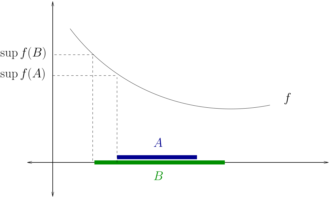
Proof

Proof, for the sup case:

Let \(A\), \(B\) and \(f\) be as in the statement of the fact

We already know that \(C \subset D \implies \sup C \leq \sup D\)

Hence it suffices to show that \(f(A) \subset f(B)\), because then

\[ % \sup_{{\bf x} \in A} f({\bf x}) := \sup f(A) \leq \sup f(B) =: \sup_{{\bf x} \in B} f({\bf x}) % \]

To see that \(f(A) \subset f(B)\), take any \(y \in f(A)\)

By definition, \(\exists \, {\bf x} \in A\) such that \(f({\bf x}) = y\)

Since \(A \subset B\) we must have \({\bf x} \in B\)

So \(f({\bf x}) = y\) for some \({\bf x} \in B\), and hence \(y \in f(B)\)

Thus \(f(A) \subset f(B)\) as was to be shown

Example

“If you have more choice then you’re better off”

Consider the problem of maximizing utility

\[ % U(x_1, x_2) = \alpha \log(x_1) + \beta \log(x_2) % \]

over all \((x_1, x_2)\) in the budget set

\[ % B(m) := \left\{ (x_1, x_2) \in \mathbb{R}^2 \;:\; x_i > 0 \text{ and } p_1 x_1 + p_2 x_2 \leq m \right\} % \]

Thus, we solve

\[ % \max_{{\bf x} \in B(m)} U({\bf x}) % \]

Clearly \(m \leq m' \implies B(m) \subset B(m')\)

Hence the maximal value goes up as \(m\) increases

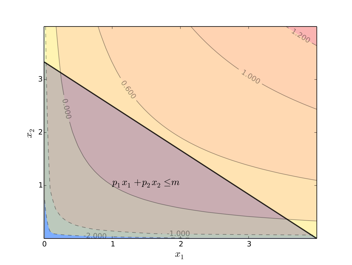
Fig. 78 Budget set \(B(m)\)

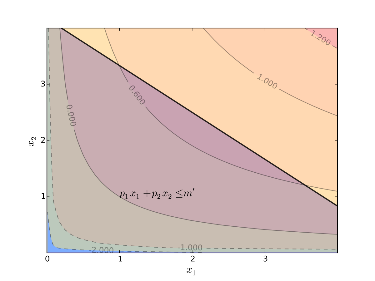
Fig. 79 Budget set \(B(m')\)

Example

Let \(y_n\) be income and \(x_n\) be years education

Consider regressing income on education:

\[ % y_n = \alpha + \beta x_n + \epsilon_n % \]

We have data for \(n = 1, \ldots, N\) individuals

Successful regression is often associated with large \(R^2\)

• A measure of “goodness of fit”

Large \(R^2\) occurs when we have a small sum of squared residuals

\[ % {\rm ssr}_a := \min_{\alpha, \beta} \; \sum_{n=1}^N \, (y_n - \alpha - \beta x_n)^2 % \]

However, we can always reduce the ssr by including irrelevant variables

• e.g., \(z_n = \) consumption of apples in kgs per annum

\[ % {\rm ssr}_b := \min_{\alpha, \beta, \gamma} \; \sum_{n=1}^N \, (y_n - \alpha - \beta x_n - \gamma z_n)^2 \, \leq {\rm ssr}_a % \]

Indeed, let

\[ % {\boldsymbol \theta} := (\alpha, \beta, \gamma), \qquad f({\boldsymbol \theta}) := \sum_{n=1}^N \, (y_n - \alpha - \beta x_n - \gamma z_n)^2 % \]

Then

\[\begin{split} % {\rm ssr}_b = \min_{{\boldsymbol \theta} \in \mathbb{R}^3} f({\boldsymbol \theta}) \leq \min_{\substack{{\boldsymbol \theta} \in \mathbb{R}^3 \\ \gamma = 0}} f({\boldsymbol \theta}) = {\rm ssr}_a % \end{split}\]

Fact

If \(f \colon A \to \mathbb{R}\), then

\[ % {\bf a}^* \in \mathrm{argmax}_{{\bf x} \in A}f({\bf x}) \; \iff \; {\bf a}^* \in \mathrm{argmin}_{{\bf x} \in A} -f({\bf x}) % \]

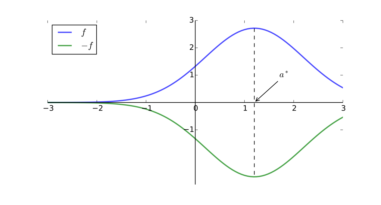
Proof

Let’s prove that, when \(g = -f\),

\[ % {\bf a}^* \in \mathrm{argmax}_{{\bf x} \in A}f({\bf x}) \; \implies \; {\bf a}^* \in \mathrm{argmin}_{{\bf x} \in A}g({\bf x}) % \]

To begin, let \({\bf a}^*\) be a maximizer of \(f\) on \(A\)

Then, for any given \({\bf x} \in A\) we have \(f({\bf a}^*) \geq f({\bf x})\)

\[ % \implies -f({\bf a}^*) \leq -f({\bf x}) % \]

\[ % \implies g({\bf a}^*) \leq g({\bf x}) % \]

Hence \({\bf a}^*\) is a minimizer of \(g\) on \(A\)

• because the last inequality was shown for any \({\bf x} \in A\)

Example

Most numerical routines provide minimization only

Suppose we want to maximize \(f(x) = 3 \ln x - x\) on \((0, \infty)\)

We can do this by finding the minimizer of \(-f\)

from scipy.optimize import fminbound
import numpy as np

f = lambda x: 3 * np.log(x) - x
g = lambda x: -f(x) # Find min of -f
print('Maximizer of f(x) on [1,100] is x=', fminbound(g, 1, 100))

Maximizer of f(x) on [1,100] is x= 3.0000015012062393

Fact

Given \(A \subset \mathbb{R}^K\), let

• \(f \colon A \to B \subset \mathbb{R}\)

• \(h \colon B \to \mathbb{R}\) and \(g := h \circ f\)

If \(h\) is strictly increasing, then

\[\mathrm{argmax}_{{\bf x} \in A}f({\bf x}) =\mathrm{argmax}_{{\bf x} \in A}g({\bf x})\]

Proof

Let \({\bf a}^* \in \mathrm{argmax}_{{\bf x} \in A}f({\bf x})\)

If \({\bf x} \in A\), then \(f({\bf x}) \leq f({\bf a}^*)\), and hence \(h(f({\bf x})) \leq h(f({\bf a}^*)) \quad\)

In other words, \(g({\bf x}) \leq g({\bf a}^*)\) for any \({\bf x} \in A\)

Hence \({\bf a}^* \in \mathrm{argmax}_{{\bf x} \in A} g({\bf x})\) as claimed

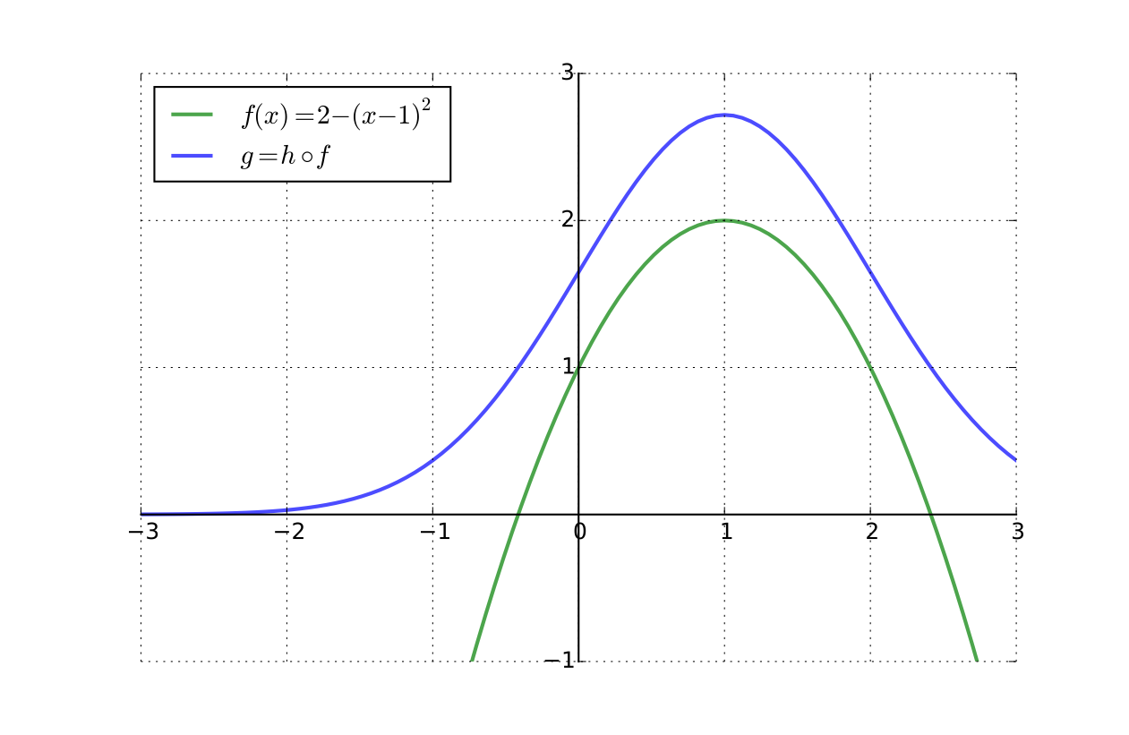
Fig. 80 Increasing transform \(h(x) = \exp(x/2)\) preserves the maximizer

Example

A well known statistical problem is to maximize the likelihood of exponential distribution:

\[ % \max_{\lambda > 0} L(\lambda) \quad \text{where} \quad L(\lambda) := \lambda^N \exp \left(-\lambda \sum_{n=1}^N x_n \right) % \]

It’s easier to maximize the log-likelihood function

\[ % \ell(\lambda) := \log(L(\lambda)) = N \log(\lambda) - \lambda \sum_{n=1}^N x_n % \]

The unique solution

\[ % \hat \lambda := \frac{N}{\sum_{n=1}^N x_n} % \]

is also the unique maximiser of \(L(\lambda)\)

In the next several propositions

• \(A\) is any set

• \(f\) is some function from \(A\) to \(\mathbb{R}\)

• \(g\) is some function from \(A\) to \(\mathbb{R}\)

To simplify notation, we define

\[ % \inf f := \inf_{{\bf x} \in A} f({\bf x}) % \]

and

\[ % \sup f := \sup_{{\bf x} \in A} f({\bf x}) % \]

Fact

\[ % f({\bf x}) \leq g({\bf x}) \text{ for all } {\bf x} \in A \implies \sup f \leq \sup g % \]

Proof

Fix any such functions \(f\) and \(g\) and any \({\bf x} \in A\)

We have

\[ % f({\bf x}) \leq g({\bf x}) \leq \sup g % \]

Hence \(\sup g\) is an upper bound for \(\{ f({\bf x}) \colon {\bf x } \in A\}\)

Since the supremum is the least upper bound, this gives

\[ % \sup f \leq \sup g % \]

Fact

\[ % \sup_{{\bf x} \in A} (f({\bf x}) + g({\bf x})) \leq \sup_{{\bf x} \in A} f({\bf x}) + \sup_{{\bf x} \in A} g({\bf x}) % \]

Proof

Fix any such functions \(f\) and \(g\) and any \({\bf x} \in A\)

We have

\[ % f({\bf x}) \leq \sup f \quad \text{and} \quad g({\bf x}) \leq \sup g % \]

\[ % \implies f({\bf x}) + g({\bf x}) \leq \sup f + \sup g % \]

\[ % \implies \sup (f + g) \leq \sup f + \sup g % \]

Fact

\[ % | \sup_{{\bf x} \in A} f({\bf x}) - \sup_{{\bf x} \in A} g({\bf x}) | \leq \sup_{{\bf x} \in A} |f({\bf x}) - g({\bf x})| % \]

Proof

Picking any such \(f, g\), we have

\[\begin{split} % \sup f = \sup (f - g + g) \leq \sup (f - g) + \sup g \\ \leq \sup | f - g | + \sup g % \end{split}\]

\[ % \text{therefore } \; \sup f - \sup g \leq \sup | f - g | % \]

Same argument reversing roles of \(f\) and \(g\) finishes the proof

Concavity and uniqueness of optima

Uniqueness of optima is directly connected to convexity / concavity

• Convexity is a shape property for sets

• Convexity and concavity are shape properties for functions

However, only one fundamental concept: convex sets

Convex Sets

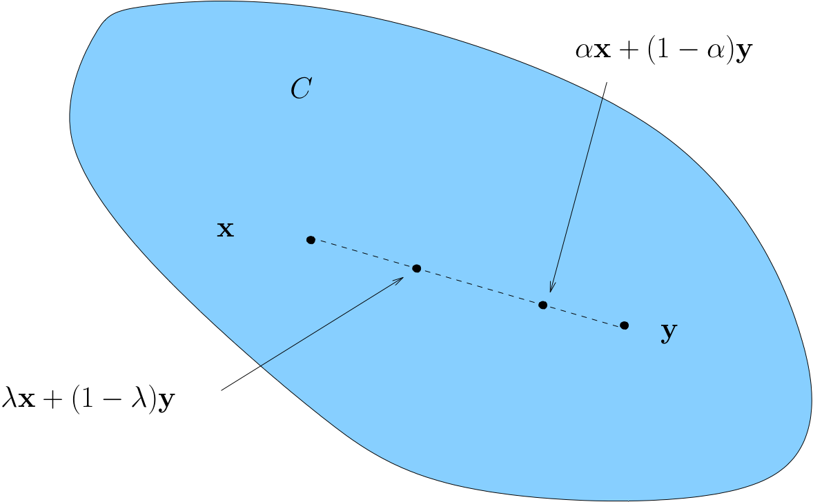
Definition

A set \(C \subset \mathbb{R}^K\) is called convex if

\[ % {\bf x}, {\bf y} \text{ in } C \text{ and } 0 \leq \lambda \leq 1 \; \implies \; \lambda {\bf x} + (1 - \lambda) {\bf y} \in C % \]

Remark: This is vector addition and scalar multiplication

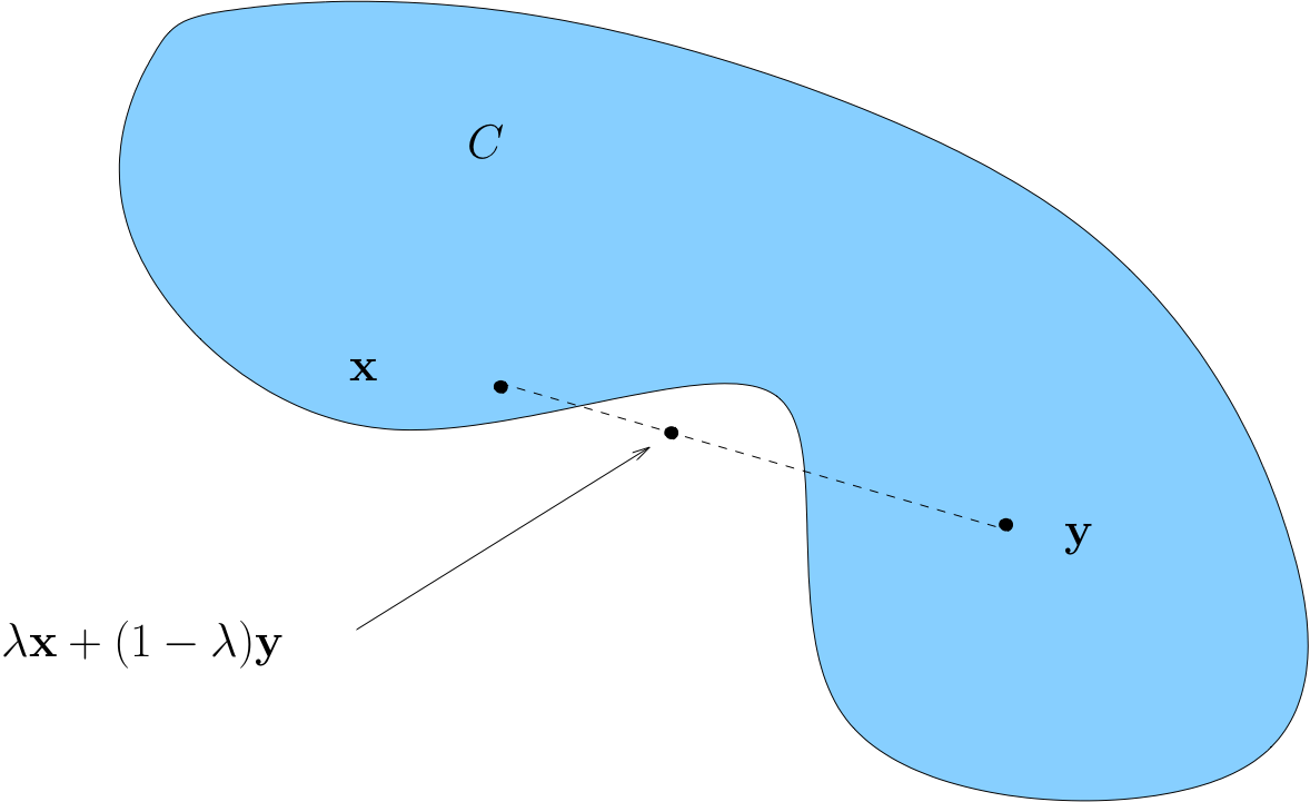
Convexity \(\iff\) line between any two points in \(C\) lies in \(C\)

A non-convex set

Example

The “positive cone” \(P := \{ {\bf x} \in \mathbb{R}^K \colon {\bf x } \geq {\bf 0} \}\) is convex

Proof

To see this, pick any \({\bf x}\), \({\bf y}\) in \(P\) and any \(\lambda \in [0, 1]\)

Let \({\bf z} := \lambda {\bf x} + (1 - \lambda) {\bf y}\) and let \(z_k := {\bf e}_k' {\bf z}\)

Since

• \(z_k = \lambda x_k + (1 - \lambda) y_k\)

• \(x_k \geq 0\) and \(y_k \geq 0\)

It is clear that \(z_k \geq 0\) for all \(k\)

Hence \({\bf z} \in P\) as claimed

Example

Every \(\epsilon\)-ball in \(\mathbb{R}^K\) is convex.

Proof

Fix \({\bf a} \in \mathbb{R}^K\), \(\epsilon > 0\) and let \(B_\epsilon({\bf a})\) be the \(\epsilon\)-ball

Pick any \({\bf x}\), \({\bf y}\) in \(B_\epsilon({\bf a})\) and any \(\lambda \in [0, 1]\)

The point \(\lambda {\bf x} + (1 - \lambda) {\bf y}\) lies in \(B_\epsilon({\bf a})\) because

\[\begin{split} % \| \lambda {\bf x} + (1 - \lambda) {\bf y} - {\bf a} \| = \| \lambda {\bf x} - \lambda {\bf a} + (1 - \lambda) {\bf y} - (1 - \lambda) {\bf a} \| \leq \\ \leq \| \lambda {\bf x} - \lambda {\bf a} \| + \| (1 - \lambda) {\bf y} - (1 - \lambda) {\bf a} \| = \\ = \lambda \| {\bf x} - {\bf a} \| + (1 - \lambda) \| {\bf y} - {\bf a} \| <> \\ < \lambda \epsilon + (1 - \lambda) \epsilon = \\ = \epsilon % \end{split}\]

Example

Let \({\bf p} \in \mathbb{R}^K\) and let \(M\) be the “half-space”

\[ % M := \{ {\bf x} \in \mathbb{R}^K \colon {\bf p }' {\bf x} \leq m\} % \]

The set \(M\) is convex

Proof

Let \({\bf p}\), \(m\) and \(M\) be as described

Fix \({\bf x}\), \({\bf y}\) in \(M\) and \(\lambda \in [0, 1]\)

Then \(\lambda {\bf x} + (1 - \lambda) {\bf y} \in M\) because

\[ % {\bf p}'[\lambda {\bf x} + (1 - \lambda) {\bf y} ] = \lambda {\bf p}'{\bf x} + (1 - \lambda) {\bf p}'{\bf y} \leq \lambda m + (1 - \lambda) m = m % \]

Hence \(M\) is convex

Fact

If \(A\) and \(B\) are convex, then so is \(A \cap B\)

Proof

Let \(A\) and \(B\) be convex and let \(C := A \cap B\)

Pick any \({\bf x}\), \({\bf y}\) in \(C\) and any \(\lambda \in [0, 1]\)

Set

\[{\bf z} := \lambda {\bf x} + (1 - \lambda) {\bf y}\]

Since \({\bf x}\) and \({\bf y}\) lie in \(A\) and \(A\) is convex we have \({\bf z} \in A\)

Since \({\bf x}\) and \({\bf y}\) lie in \(B\) and \(B\) is convex we have \({\bf z} \in B\)

Hence \({\bf z} \in A \cap B\)

Example

Let \({\bf p} \in \mathbb{R}^K\) be a vector of prices and consider the budget set

\[ % B(m) := \{ {\bf x} \in \mathbb{R}^K \colon {\bf x } \geq {\bf 0} \text{ and } {\bf p}' {\bf x} \leq m\} % \]

The budget set \(B(m)\) is convex

Proof

To see this, note that \(B(m) = P \cap M\) where

\[ % P := \{ {\bf x} \in \mathbb{R}^K \colon {\bf x } \geq {\bf 0} \} \qquad M := \{ {\bf x} \in \mathbb{R}^K \colon {\bf p }' {\bf x} \leq m\} % \]

We already know that

• \(P\) and \(M\) are convex, intersections of convex sets are convex

Hence \(B(m)\) is convex

Convex Functions

Let \(A \subset \mathbb{R}^K\) be a convex set and let \(f\) be a function from \(A\) to \(\mathbb{R}\)

Definition

\(f\) is called convex if

\[ % f(\lambda {\bf x} + (1 - \lambda) {\bf y}) \leq \lambda f({\bf x}) + (1 - \lambda) f({\bf y}) % \]

for all \({\bf x}, {\bf y} \in A\) and all \(\lambda \in [0, 1]\)

Definition

\(f\) is called strictly convex if

\[ % f(\lambda {\bf x} + (1 - \lambda) {\bf y}) < \lambda f({\bf x}) + (1 - \lambda) f({\bf y}) % \]

for all \({\bf x}, {\bf y} \in A\) with \({\bf x} \ne {\bf y}\) and all \(\lambda \in (0, 1)\)

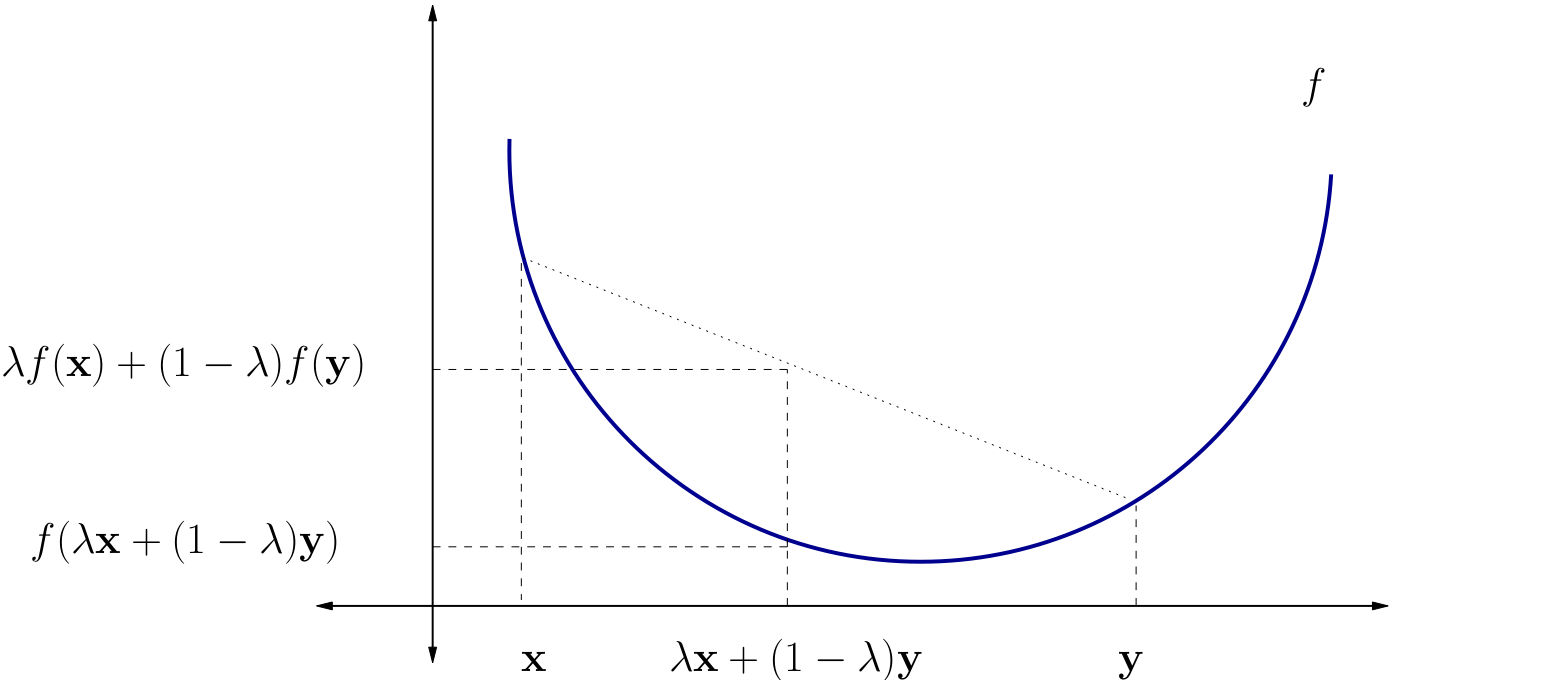
Fig. 81 A strictly convex function on a subset of \(\mathbb{R}\)

Fact

\(f \colon A \to \mathbb{R}\) is convex if and only if its epigraph (aka supergraph)

\[ % E_f := \{ ({\bf x}, y) \in A \times \mathbb{R} \colon f({\bf x \}) \leq y} % \]

is a convex subset of \(\mathbb{R}^K \times \mathbb{R}\)

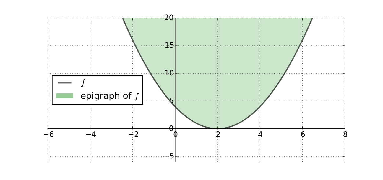
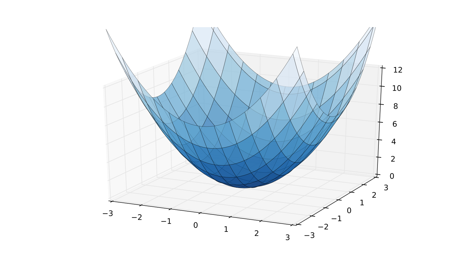
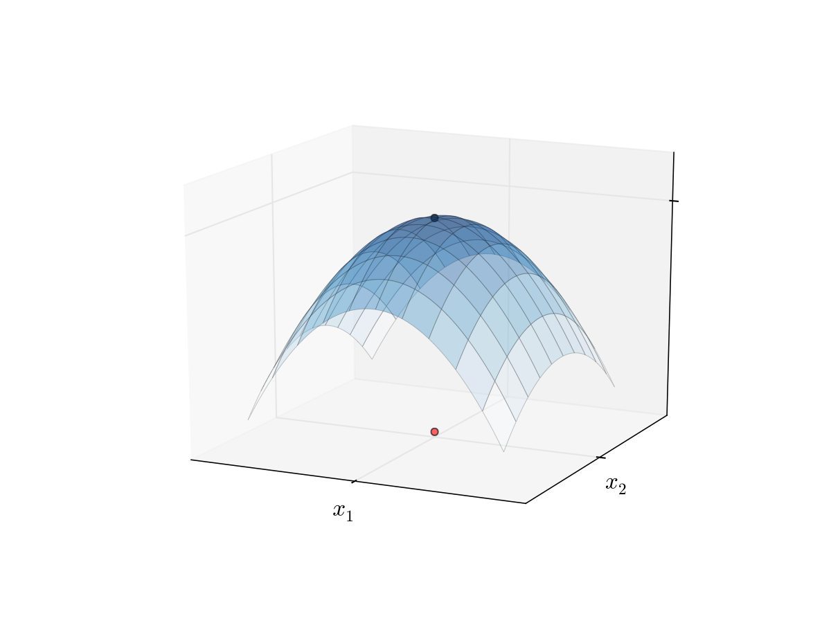
Fig. 82 A strictly convex function on a subset of \(\mathbb{R}^2\)

Example

\(f({\bf x}) = \|{\bf x}\|\) is convex on \(\mathbb{R}^K\)

Proof

To see this recall that, by the properties of norms,

\[\begin{split} % \|\lambda {\bf x} + (1 - \lambda) {\bf y}\| \leq \|\lambda {\bf x}\| + \|(1 - \lambda) {\bf y}\| \\ = \lambda \|{\bf x}\| + (1 - \lambda) \|{\bf y}\| % \end{split}\]

That is,

\[ % f(\lambda {\bf x} + (1 - \lambda) {\bf y}) \leq \lambda f({\bf x}) + (1 - \lambda) f({\bf y}) % \]

Example

\(f(x) = \cos(x)\) is not convex on \(\mathbb{R}\) because

\[ % 1 = f(2\pi) = f(\pi/2 + 3\pi/2) > f(\pi)/2 + f(3\pi)/2 = -1 % \]

Fact

If \({\bf A}\) is \(K \times K\) and positive definite, then

\[ % Q({\bf x}) = {\bf x}' {\bf A} {\bf x} \qquad ({\bf x} \in \mathbb{R}^K) % \]

is strictly convex on \(\mathbb{R}^K\)

Proof

Proof: Fix \({\bf x}, {\bf y} \in \mathbb{R}^K\) with \({\bf x} \ne {\bf y}\) and \(\lambda \in (0, 1)\)

Exercise: Show that

\[\begin{split} % \lambda Q({\bf x}) + (1 - \lambda) Q({\bf y}) - Q(\lambda {\bf x} + (1 - \lambda) {\bf y}) \\ = \lambda (1 - \lambda) ({\bf x} - {\bf y})' {\bf A} ({\bf x} - {\bf y}) % \end{split}\]

Since \({\bf x} - {\bf y} \ne {\bf 0}\) and \(0 < \lambda < 1\), the right hand side is \(> 0\)

Hence

\[ % \lambda Q({\bf x}) + (1 - \lambda) Q({\bf y}) > Q(\lambda {\bf x} + (1 - \lambda) {\bf y}) % \]

Concave Functions

Let \(A \subset \mathbb{R}^K\) be a convex and let \(f\) be a function from \(A\) to \(\mathbb{R}\)

Definition

\(f\) is called concave if

\[ % f(\lambda {\bf x} + (1 - \lambda) {\bf y}) \geq \lambda f({\bf x}) + (1 - \lambda) f({\bf y}) % \]

for all \({\bf x}, {\bf y} \in A\) and all \(\lambda \in [0, 1]\)

Definition

\(f\) is called strictly concave if

\[ % f(\lambda {\bf x} + (1 - \lambda) {\bf y}) > \lambda f({\bf x}) + (1 - \lambda) f({\bf y}) % \]

for all \({\bf x}, {\bf y} \in A\) with \({\bf x} \ne {\bf y}\) and all \(\lambda \in (0, 1)\)

Exercise: Show that

1. \(f\) is concave if and only if \(-f\) is convex

2. \(f\) is strictly concave if and only if \(-f\) is strictly convex

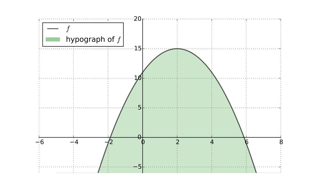
Fact

\(f \colon A \to \mathbb{R}\) is concave if and only if its hypograph (aka subgraph)

\[ % H_f := \{ ({\bf x}, y) \in A \times \mathbb{R} \colon f({\bf x \}) \geq y} % \]

is a convex subset of \(\mathbb{R}^K \times \mathbb{R}\)

Preservation of Shape

Let \(A \subset \mathbb{R}^K\) be convex and let \(f\) and \(g\) be functions from \(A\) to \(\mathbb{R}\)

Fact

If \(f\) and \(g\) are convex (resp., concave) and \(\alpha \geq 0\), then

• \(\alpha f\) is convex (resp., concave)

• \(f + g\) is convex (resp., concave)

Fact

If \(f\) and \(g\) are strictly convex (resp., strictly concave) and \(\alpha > 0\), then

• \(\alpha f\) is strictly convex (resp., strictly concave)

• \(f + g\) is strictly convex (resp., strictly concave)

Let’s prove that \(f\) and \(g\) convex \(\implies h := f + g\) convex

Pick any \({\bf x}, {\bf y} \in A\) and \(\lambda \in [0, 1]\)

We have

\[\begin{split} % & h(\lambda {\bf x} + (1 - \lambda) {\bf y}) = f(\lambda {\bf x} + (1 - \lambda) {\bf y}) + g(\lambda {\bf x} + (1 - \lambda) {\bf y}) \\ & \leq \lambda f({\bf x}) + (1 - \lambda) f({\bf y}) + \lambda g({\bf x}) + (1 - \lambda) g({\bf y}) \\ & = \lambda [f({\bf x}) + g({\bf x})] + (1 - \lambda) [f({\bf y}) + g({\bf y})] \\ & = \lambda h({\bf x}) + (1 - \lambda) h({\bf y}) % \end{split}\]

Hence \(h\) is convex

Uniqueness of Optimizers

Fact

Let \(A \subset \mathbb{R}^K\) be convex and let \(f \colon A \to \mathbb{R}\)

1. If \(f\) is strictly convex, then \(f\) has at most one minimizer on \(A\)

2. If \(f\) is strictly concave, then \(f\) has at most one maximizer on \(A\)

Interpretation, strictly concave case:

• we don’t know in general if \(f\) has a maximizer

• but if it does, then it has exactly one

• in other words, we have uniqueness

Proof

Proof for the case where \(f\) is strictly concave:

Suppose to the contrary that

• \({\bf a}\) and \({\bf b}\) are distinct points in \(A\)

• both are maximizers of \(f\) on \(A\)

By the def of maximizers, \(f({\bf a}) \geq f({\bf b})\) and \(f({\bf b}) \geq f({\bf a})\)

Hence we have \(f({\bf a}) = f({\bf b})\)

By strict concavity, then

\[ % f\left( \frac{1}{2} {\bf a} + \frac{1}{2} {\bf b} \right) > \frac{1}{2} f( {\bf a}) + \frac{1}{2} f( {\bf b}) = \frac{1}{2} f( {\bf a}) + \frac{1}{2} f( {\bf a}) = f({\bf a}) % \]

This contradicts the assumption that \({\bf a}\) is a maximizer

A Sufficient Condition

We can now restate more precisely optimization results stated in the introductory lectures

Let \(f \colon A \to \mathbb{R}\) be a \(C^2\) function where \(A \subset \mathbb{R}^K\) is open, convex

Recall that \({\bf x}^* \in A\) is a stationary point of \(f\) if

\[ % \frac{\partial}{\partial x_i} f({\bf x}^*) = 0 \quad \text{for all $i$ in } 1, \ldots, K % \]

Fact

If \(f\) and \(A\) are as above and \({\bf x}^* \in A\) is stationary, then

1. \(f\) strictly concave \(\implies\) \({\bf x}^*\) is the unique maximizer of \(f\) on \(A\)

2. \(f\) strictly convex \(\implies\) \({\bf x}^*\) is the unique minimizer of \(f\) on \(A\)