Unconstrained optimization

ECON2125/6012 Lecture 7 Fedor Iskhakov

Announcements & Reminders

• Test 2 results and discussion

• Exam is preliminary scheduled to Monday, 6 November 9:00 to 12:15

Plan for this lecture

1. Optimization problems in economics

2. Multivariate calculus

3. Necessary (first order) condition in \(\mathbb{R}^n\)

4. Sufficient (second order) and shape conditions

Supplementary reading:

• Simon & Blume: 13.1, 13.2, 13.3, 14.1, 14.3, 14.4, 14.5, 14.8, whole of chapter 17

• Sundaram: 1.4, 1.5, 2.1, 2.2, 4.1 to 4.4

An optimization problem

Example

Consider a (monopolistic) firm that is facing a market demand for its products \(D(p) = \alpha + \frac{1}{4\alpha}p^2-p\) and the cost of production \(C(q) = \beta q + \delta q^2\). As usual, \(p\) and \(q\) denote price and quantity of product, respectively.

To maximize its profit \(\pi(p,q) = pq-C(q)\), the firm solves the following optimization problem

\[\begin{split} \Pi(\alpha,\beta,\delta) = \max_{p,q} \pi(p,q) = \max_{p,q} \big[ p q - C(q) \big] \\ \text {subject to} \\ q = D(p)\\ q \ge 0\\ p > 0 \end{split}\]

Plugging in the functions \(D(p)\) and \(C(q)\) we have an equivalent formulation

\[\begin{split} \Pi(\alpha,\beta,\delta) = \max_{p,q} \big[ (p-\beta) q - \delta q^2 \big] \\ \text {subject to} \\ q = \alpha + \frac{1}{4\alpha}p^2-p\\ q \ge 0\\ p > 0 \end{split}\]

Components of the optimization problem

1. Objective function: function to be maximized or minimized, also known as maximand
   In the example above profit function \(\pi(p,q) = pq - C(q)\) to be maximized

2. Decision/choice variables: the variables that the agent can control in order to optimize the objective function, also known as controls
   In the example above price \(p\) and quantity \(q\) variables that the firm can choose to maximize its profit

3. Equality constraints: restrictions on the choice variables in the form of equalities
   In the example above \(q = \alpha + \frac{1}{4\alpha}p^2-p\)

4. Inequality constraints (weak and strict): restrictions on the choice variables in the form of inequalities
   In the example above \(q \ge 0\) and \(p > 0\)

5. Parameters: the variables that are not controlled by the agent, but affect the objective function and/or constraints
   In the example above \(\alpha\), \(\beta\) and \(\delta\) are parameters of the problem

6. Value function: the “optimized” value of the objective function as a function of parameters
   In the example above \(\Pi(\alpha,\beta,\delta)\) is the value function

Definition

The general form of the optimization problem is

\[\begin{split} V(\theta) = \max_{x} f(x,\theta) \\ \text {subject to} \\ g_i(x,\theta) = 0, \; i\in\{1,\dots,I\}\\ h_j(x,\theta) \le 0, \; j\in\{1,\dots,J\} \end{split}\]

where:

• \(f(x,\theta) \colon \mathbb{R}^N \times \mathbb{R}^K \to \mathbb{R}\) is an objective function

• \(x \in \mathbb{R}^N\) are decision/choice variables

• \(\theta \in \mathbb{R}^K\) are parameters

• \(g_i(x,\theta) = 0, \; i\in\{1,\dots,I\}\) where \(g_i \colon \mathbb{R}^N \times \mathbb{R}^K \to \mathbb{R}\), are equality constraints

• \(h_j(x,\theta) \le 0, \; j\in\{1,\dots,J\}\) where \(h_j \colon \mathbb{R}^N \times \mathbb{R}^K \to \mathbb{R}\), are inequality constraints

• \(V(\theta) \colon \mathbb{R}^K \to \mathbb{R}\) is a value function

Definition

The set of admissible choices (admissible set) contains all the choices that satisfy the constraints of the optimization problem.

Note

Sometimes the equality constraints are dropped from the definition of the optimization problem, because they can always be represented as a pair of inequality constraints \(g_i(x,\theta) \le 0\) and \(-g_j(x,\theta) \le 0\)

Note

Note that strict inequality constraints are not present in the definition above, although they may be present in the economic applications. You already know that this has to do with the intention to keep the set of admissible choices closed, such that the solution of the problem (has a better chance to) exist. Sometimes they are added to the definition.

A roadmap for formulating an optimization problem (in economics)

1. Determine which variables are choice variables and which are parameters according to what the economic agent has control over

2. Determine whether the optimization problem is a maximization or a minimization problem

3. Determine the objective function of the economic agent (and thus the optimization problem)

4. Determine the constraints of the optimization problem: equality and inequality, paying particular attention to whether inequalities should be strict or weak (the latter has huge implications for the existence of the solution)

Example

Consider a decision maker who is deciding how to divide the money they have between food and services, bank deposit and buying some crypto. Discuss and Write down the corresponding optimization problem. [class exercise]

Classes of the optimization problems

1. Static optimization: finite number of choice variables

• singe instance of choice

• deterministic finite horizon dynamic choice models can be represented as static

• our main focus in this course

2. Dynamic programming: some choice variables are infinite sequences, solved using similar techniques as static optimization

• will touch upon in the end of the course

3. Deterministic optimal control: some “choice variables” are functions, completely new theory is needed

4. Stochastic optimal control: “choice variables” are functions, objective function is a stochastic process, yet more theory is needed

Review of one-dimensional optimization

Let \(f \colon [a, b] \to \mathbb{R}\) be a differentiable function

• \(f\) takes \(x \in [a, b] \subset \mathbb{R}\) and returns number \(f(x)\)

• derivative \(f'(x)\) exists for all \(x\) with \(a < x < b\)

Differentiability implies that \(f\) is continuous, and because the interval \([a,b]\) is closed and bounded, \(f\) has a maximum and a minimum on \([a,b]\) by the Weierstrass extreme value theorem.

Reminder of definitions

A point \(x^* \in [a, b]\) is called a

• maximizer of \(f\) on \([a, b]\) if \(f(x^*) \geq f(x)\) for all \(x \in [a,b]\)

• minimizer of \(f\) on \([a, b]\) if \(f(x^*) \leq f(x)\) for all \(x \in [a,b]\)

Point \(x\) is called interior to \([a, b]\) if \(a < x < b\)

A stationary point of \(f\) on \([a, b]\) is an interior point \(x\) with \(f'(x) = 0\)

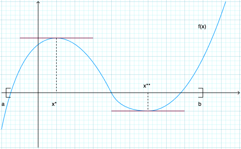
Fig. 83 Both \(x^*\) and \(x^{**}\) are stationary

Fact

If \(f\) is differentiable and \(x^*\) is either an interior minimizer or an interior maximizer of \(f\) on \([a, b]\), then \(x^*\) is stationary

\(\Rightarrow\) any interior maximizer stationary
\(\Rightarrow\) set of interior maximizers \(\subset\) set of stationary points
\(\Rightarrow\) maximizers \(\subset \text{stationary points} \cup \{a\} \cup \{b\}\)

Algorithm for finding maximizers/minimizers:

1. Locate stationary points

2. Evaluate \(y = f(x)\) for each stationary \(x\) and for \(a\), \(b\)

3. Pick point giving largest \(y\) value

Sufficiency and uniqueness with shape conditions

Fact

Sufficient conditions for concavity in one dimension

Let \(f \colon [a, b] \to \mathbb{R}\)

• If \(f''(x) \leq 0\) for all \(x \in (a, b)\) then \(f\) is concave on \((a, b)\)

• If \(f''(x) < 0\) for all \(x \in (a, b)\) then \(f\) is strictly concave on \((a, b)\)

Sufficient conditions for convexity in one dimension

Let \(f \colon [a, b] \to \mathbb{R}\)

• If \(f''(x) \geq 0\) for all \(x \in (a, b)\) then \(f\) is convex on \((a, b)\)

• If \(f''(x) > 0\) for all \(x \in (a, b)\) then \(f\) is strictly convex on \((a, b)\)

Fact

For maximizers:

• If \(f \colon [a,b] \to \mathbb{R}\) is concave and \(x^* \in (a, b)\) is stationary then \(x^*\) is a maximizer

• If, in addition, \(f\) is strictly concave, then \(x^*\) is the unique maximizer

For minimizers:

• If \(f \colon [a,b] \to \mathbb{R}\) is convex and \(x^* \in (a, b)\) is stationary then \(x^*\) is a minimizer

• If, in addition, \(f\) is strictly convex, then \(x^*\) is the unique minimizer

Let us generalize these results to the multivariate case.

Multivariate calculus

Reminder of the derivative in one dimension

Let \(f \colon (a, b) \to \mathbb{R}\) and let \(x \in (a, b)\)

Let \(H\) be all sequences \(\{h_n\}\) such that \(h_n \ne 0\) and \(h_n \to 0\)

If there exists a constant \(f'(x)\) such that

\[ \frac{f(x + h_n) - f(x)}{h_n} \to f'(x) \]

for every \(\{h_n\} \in H\), then

• \(f\) is said to be differentiable at \(x\)

• \(f'(x)\) is called the derivative of \(f\) at \(x\)

In higher dimensions this definition has to be adjusted to account for the fact that \(h_n\) is a vector in \(\mathbb{R}^N\)

Definition

Let

• \(A \subset \mathbb{R}^N\) be an open set in \(N\)-dimensional space.

• \(f \colon A \to \mathbb{R}^K\) be a \(K\) dimensional vector function

• \({\bf x} \in A\), and so \(\exists \epsilon \colon B_{\epsilon}({\bf x}) \subset A\)

Then if there exists a \(K \times N\) matrix \(J\) such that

\[ \frac{\|f({\bf x} + {\bf h}_n) - f({\bf x}) - J {\bf h}_n\|}{\|{\bf h}_n\|} \to 0 \]

for all converging to zero sequences \(\{{\bf h}_n\}\), \({\bf h}_n \in B_{\epsilon}({\bf 0}) \setminus \{{\bf 0}\}\), \({\bf h}_n \to {\bf 0}\), then

• \(f\) is said to be differentiable at \({\bf x}\)

• matrix \(J\) is called the total derivative (or Jacobian matrix) of \(f\) at \({\bf x}\), and is denoted by \(Df({\bf x})\) or simply \(f'({\bf x})\)

Note

The vector function \(f \colon \mathbb{R}^N \to \mathbb{R}^K\) (also known as vector-valued function) can be thought of as a tuple of \(K\) functions \(f_j \colon \mathbb{R}^N \to \mathbb{R}\), \(j \in \{1, \dots, K\}\)

Contrast the definition of total derivative to the definition of the partial derivative

Definition

Let \(f \colon A \to \mathbb{R}\) and let \({\bf x} \in A \subset \mathbb{R}^N\). Denote \({\bf e}_i\) the \(i\)-th unit vector in \(\mathbb{R}^N\), i.e. \({\bf e}_i = (0, \dots, 0, 1, 0, \dots, 0)\) where \(1\) is in the \(i\)-th position.

If there exists a constant \(a \in \mathbb{R}\) such that

\[ \frac{\| f({\bf x} + h_n {\bf e}_i) - f({\bf x})\|}{h_n} \to a \]

for every sequence \(\{h_n\}\), \(h_n \in \mathbb{R}\), such that \(h_n \ne 0\) and \(h_n \to 0\) as \(n \to \infty\), then \(a\) is called a partial derivative of \(f\) with respect to \(x_i\) at \({\bf x}\), and is denoted \(f'_i({\bf x})\) or \(\frac{\partial f}{\partial x_i}({\bf x})\)

Total derivative of \(f \colon \mathbb{R}^N \to \mathbb{R}^K\) defines a linear map \(J \colon \mathbb{R}^N \to \mathbb{R}^K\) given by \(K \times N\) matrix \(Df(x)\) which gives a affine approximation of function \(f\) by a tangent hyperplane at point \({\bf x}\). This is similar to the tangent line to a one-dimensional function determined by a derivative at any given point.

Fact

If a vector function \(f \colon \mathbb{R}^N \to \mathbb{R}^K\) is differentiable at \({\bf x}\), then all partial derivatives at \({\bf x}\) exist and the total derivative (Jacobian) is given by

\[\begin{split} Df({\bf x}) = \left( \begin{array}{ccc} \frac{\partial f_1}{\partial x_1}({\bf x}) & \cdots & \frac{\partial f_1}{\partial x_N}({\bf x}) \\ \vdots & \ddots & \vdots \\ \frac{\partial f_K}{\partial x_1}({\bf x}) & \cdots & \frac{\partial f_K}{\partial x_N}({\bf x}) \end{array} \right) \end{split}\]

Fact

If all partial derivatives of \(f \colon \mathbb{R}^N \to \mathbb{R}^K\) exist and are continuous in \({\bf x}\), then \(f\) is differentiable at \({\bf x}\)

The last two facts can be stated for sets by adding the condition that the statements hold in all elements on the sets (such as “for all \({\bf x} \in A\)”)

Example

\[\begin{split} f \colon \left( \begin{array}{c} x_1 \\ x_2 \\ x_3 \end{array} \right) \mapsto \left( \begin{array}{l} x_1^2 + x_2 x_3 \\ x_1+x_2^2+x_3^3 \end{array} \right) \end{split}\]

Partial derivatives are

\[ \frac{\partial f_1}{\partial x_1} = 2 x_1, \; \frac{\partial f_1}{\partial x_2} = x_3, \; \frac{\partial f_1}{\partial x_3} = x_2 \]

\[ \frac{\partial f_2}{\partial x_1} = 1, \; \frac{\partial f_2}{\partial x_2} = 2x_2, \; \frac{\partial f_2}{\partial x_3} = 3x_3^2 \]

Jacobian matrix is

\[\begin{split} Df({\bf x}) = \left( \begin{array}{rrr} 2x_1, & x_3, & x_2 \\ 1, & 2x_2, & 3x_3^2 \end{array} \right) \end{split}\]

Now, evaluating at a particular points

\[\begin{split} Df({\bf 0}) = \left( \begin{array}{rrr} 0, & 0, & 0 \\ 1, & 0, & 0 \end{array} \right) \end{split}\]

\[\begin{split} Df({\bf 1}) = \left( \begin{array}{rrr} 2, & 1, & 1 \\ 1, & 2, & 3 \end{array} \right) \end{split}\]

\[\begin{split} Df((1,2,3)') = \left( \begin{array}{rrr} 2, & 3, & 2 \\ 1, & 4, & 27 \end{array} \right) \end{split}\]

Example

\[\begin{split} f \colon \left( \begin{array}{c} x_1 \\ x_2 \\ x_3 \end{array} \right) \mapsto \left( \begin{array}{l} x_1 + x_1 x_2 x_3 \\ x_1+2x_2-x_3 \\ x_1+2x_3 \\ x_2x_3 \end{array} \right) \end{split}\]

Exercise: Derive Jacobian maxtix of \(f\) and compute the total derivative of \(f\) at \({\bf x} = (1, 0, 2)\)

Definition

For a function \(f \colon \mathbb{R}^N \to \mathbb{R}\) the Jacobian matrix takes is \(1 \times N\) vector which is called gradient and is often denoted \(\nabla f({\bf x}) \in \mathbb{R}^N\)

\[ \nabla f({\bf x}) = \left(\frac{\partial f}{\partial x_1}, \dots, \frac{\partial f}{\partial x_N} \right) \in \mathbb{R}^N \]

Rules of differentiation

Fact

Let \(A\) denote an open set in \(\mathbb{R}^N\) and let \(f, g \colon A \to \mathbb{R}^K\) be differentiable functions at \({\bf x} \in A\).

1. \(f+g\) is differentiable at \({\bf x}\) and \(D(f+g)({\bf x}) = Df({\bf x}) + Dg({\bf x})\)

2. \(cf\) is differentiable at \({\bf x}\) and \(D(cf)({\bf x}) = c Df({\bf x})\) for any scalar \(c\)

Fact: Product (Leibniz) rule

Let \(A\) denote an open set in \(\mathbb{R}^N\) and let \(f \colon A \to \mathbb{R}\) and \(g \colon A \to \mathbb{R}^K\) be both differentiable functions at \({\bf x} \in A\).

Then \(f g\) is differentiable at \({\bf x}\) and \(D(f g)({\bf x}) = f({\bf x}) Dg({\bf x}) + g({\bf x}) \nabla f({\bf x})\)

Fact: Dot product rule

Let \(A\) denote an open set in \(\mathbb{R}^N\) and let \(f,g \colon A \to \mathbb{R}^K\) be both differentiable functions at \({\bf x} \in A\).

Then \(f \cdot g\) is differentiable at \({\bf x}\) and \(D(f \cdot g)({\bf x}) = [f({\bf x})]' Dg({\bf x}) + [g({\bf x})]' Df({\bf x})\), where \([\cdot]'\) denotes vector transpose

Fact: Chain rule

Let \(A\) denote an open set in \(\mathbb{R}^N\) and \(C\) denote an open set in \(\mathbb{R}^K\). Let \(f \colon A \to C\) be differentiable at \({\bf x} \in A\), and \(g \colon C \to \mathbb{R}^L\) be differentiable at \(f({\bf x}) \in C\).

Then the composition \(g \circ f\) is differentiable at \({\bf x}\) and its total derivatibe is given by \(D(g \circ f)({\bf x}) = Dg(f({\bf x})) Df({\bf x})\)

Example

\[\begin{split} f \colon \left( \begin{array}{c} x_1 \\ x_2 \\ x_3 \end{array} \right) \mapsto \left( \begin{array}{l} x_1^3 + x_2 x_3 \\ x_2+x_1 x_3^2 \end{array} \right) \end{split}\]

\[\begin{split} Df({\bf x}) = \left( \begin{array}{lll} 3x_1^2, & x_3, & x_2 \\ x_3^2, & 1, & 2x_1x_3 \end{array} \right) \end{split}\]

\[\begin{split} g \colon \left( \begin{array}{c} y_1 \\ y_2 \end{array} \right) \mapsto \left( \begin{array}{l} 2 y_1^2 \\ y_1 + y_2 \\ y_1 - y_2 \\ 4 y_2^2 \\ \end{array} \right) \end{split}\]

\[\begin{split} Dg({\bf y}) = \left( \begin{array}{lll} 4y_1, & 0 \\ 1, & 1 \\ 1, & -1 \\ 0, & 8y_2 \end{array} \right) \end{split}\]

Applying the chain rule

\[\begin{split} D(g \circ f)({\bf x}) = \left( \begin{array}{lll} 4(x_1^3 + x_2 x_3), & 0 \\ 1, & 1 \\ 1, & -1 \\ 0, & 8(x_2+x_1 x_3^2) \end{array} \right) \left( \begin{array}{lll} 3x_1^2, & x_3, & x_2 \\ x_3^2, & 1, & 2x_1x_3 \end{array} \right) \end{split}\]

\[\begin{split} D(g \circ f)({\bf x}) = \left( \begin{array}{lll} 12x_1^2(x_1^3 + x_2 x_3), & 4x_3(x_1^3 + x_2 x_3), & 4x_2(x_1^3 + x_2 x_3)\\ 3x_1^2+x_3^2, & x_3+1, & x_2+2x_1x_3 \\ 3x_1^2-x_3^2, & x_3-1, & x_2-2x_1x_3 \\ 8x_3^2(x_2+x_1 x_3^2), & 8(x_2+x_1 x_3^2), & 16 x_1 x_3(x_2+x_1 x_3^2) \end{array} \right) \end{split}\]

Now we can evaluate \(D(g \circ f)({\bf x})\) at a particular points in \(\mathbb{R}^3\)

Example

\[\begin{split} f \colon \left( \begin{array}{c} x_1 \\ x_2 \end{array} \right) \mapsto \left( \begin{array}{l} x_1^2 + x_2^2 \\ x_1 x_2 \end{array} \right) \end{split}\]

\[\begin{split} g \colon \left( \begin{array}{c} y_1 \\ y_2 \end{array} \right) \mapsto (y_1+2 y_2)^2 \end{split}\]

Exercise: Using the chain rule, find the total derivative of the composition \(g \circ f\).

• The chain rule very powerful tool in computing complex derivatives (think backwards propagation in deep neural networks)

Higher order derivatives

The higher order derivatives of the function in one dimension generalize naturally to the multivariate case, but the complexity of the needed matrixes and multidimensional arrays (tensors) grows fast.

Definition

Let \(A\) denote an open set in \(\mathbb{R}^N\), and let \(f \colon A \to \mathbb{R}\). Assume that \(f\) is twice differentiable at \({\bf x} \in A\).

The total derivative of the gradient of function \(f\) at point \({\bf x}\), \(\nabla f({\bf x})\) is called the Hessian matrix of \(f\) denoted by \(Hf\) or \(\nabla^2 f\), and is given by a \(N \times N\) matrix

\[\begin{split} Hf({\bf x}) = \nabla^2 f({\bf x}) = \left( \begin{array}{ccc} \frac{\partial^2 f}{\partial x_1 \partial x_1}({\bf x}) & \cdots & \frac{\partial^2 f}{\partial x_1 \partial x_N}({\bf x}) \\ \vdots & \ddots & \vdots \\ \frac{\partial^2 f}{\partial x_N \partial x_1}({\bf x}) & \cdots & \frac{\partial^2 f}{\partial x_N \partial x_N}({\bf x}) \end{array} \right) \end{split}\]

Fact

For every \({\bf x} \in A \subset \mathbb{R}^N\) where \(A\) is an open and \(f \colon A \to \mathbb{R}^N\) is twice continuously differentiable, the Hessian matrix \(\nabla^2 f({\bf x})\) is symmetric

Example

\[\begin{split} f \colon \left( \begin{array}{c} x_1 \\ x_2 \end{array} \right) \mapsto (x_1 - 2 x_2)^2 \end{split}\]

\[\begin{split} \nabla^2 f({\bf x}) = \left( \begin{array}{rr} 2, & -4 \\ -4, & 8 \end{array} \right) \end{split}\]

Exercise: check

Example

\[\begin{split} f \colon \left( \begin{array}{c} x_1 \\ x_2 \end{array} \right) \mapsto (x_1 - 2 x_2)^3 \end{split}\]

\[\begin{split} \nabla^2 f({\bf x}) = 6 (x_1 - 2 x_2) \left( \begin{array}{rr} 1, & -2 \\ -2, & 4 \end{array} \right) \end{split}\]

Exercise: check

First oder conditions (FOC), necessary

In this lecture we focus on the unconstrained optimization problems of the form

\[\begin{split} \max_{x} f(x,\theta) \text{ also written as } f(x,\theta) \rightarrow \max,\\ \min_{x} f(x,\theta) \text{ also written as } f(x,\theta) \rightarrow \min, \end{split}\]

where \(f(x,\theta) \colon \mathbb{R}^N \to \mathbb{R}\) and unless stated otherwise is assumed to be continuous and twice continuously differentiable everywhere on \(\mathbb{R}^N\). Parameter \(\theta\) may or may not be present.

Note

Twice continuously differentiable functions are said to be \(C^2\).

• Every point in the whole space \(\mathbb{R}^N\) is interior, therefore all maximizers/minimizers have to be stationary points

• Assuming differentiability implies we can focus on derivative based conditions

Definition

Given a function \(f \colon \mathbb{R}^N \to \mathbb{R}\), a point \({\bf x} \in \mathbb{R}^N\) is called a stationary point of \(f\) if \(\nabla f({\bf x}) = {\bf 0}\)

Definition

Given a function \(f \colon \mathbb{R}^N \to \mathbb{R}\), a point \({\bf x^\star} \in \mathbb{R}^N\) is called a local maximizer/minimizer of \(f\) if \(\exists \epsilon\) such that \(f({\bf x}) \le f({\bf x^\star})\) for all \(x \in B_{\epsilon}({\bf x^\star})\)

If the inequality is strict, then \({\bf x^\star}\) is called a strict local maximizer/minimizer of \(f\)

A maximizer/minimizer (global) must also be a local one, but the opposite is not necessarily true.

Fact (Necessary condition for optima)

Let \(f(x,\theta) \colon \mathbb{R}^N \to \mathbb{R}\) be a differentiable function and let \({\bf x^\star} \in \mathbb{R}^N\) be a local maximizer/minimizer of \(f\).

Then \({\bf x^\star}\) is a stationary point of \(f\), that is \(\nabla f({\bf x^\star}) = {\bf 0}\)

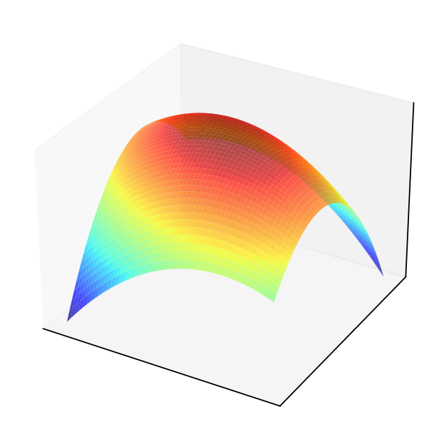
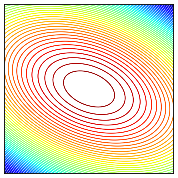
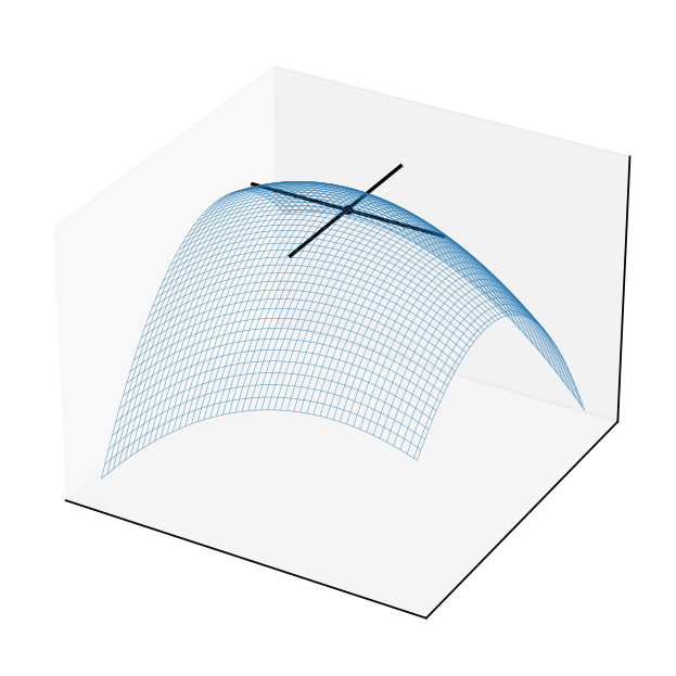
Example

Consider quadratic form \(f({\bf x}) = {\bf x}' A {\bf x}\) where \(A = \left( \begin{array}{rr} 1,& 0.5 \\ 0.5,& 2 \end{array} \right)\)

Solving the FOC

\[ \nabla f({\bf x}) = 2 {\bf x}' A = 0 \implies {\bf x} = {\bf 0} \]

The point \((0,0)\) should be an optimizer.

Show code cell source Hide code cell source

import numpy as np
import matplotlib.pyplot as plt
from mpl_toolkits.mplot3d import Axes3D
from matplotlib import cm

A = np.array([[1,.5],[.5,2]])
f = lambda x: -(x@A@x)
x = y = np.linspace(-5.0, 5.0, 100)
X, Y = np.meshgrid(x, y)
zs = np.array([f((x,y)) for x,y in zip(np.ravel(X), np.ravel(Y))])
Z = zs.reshape(X.shape)

fig = plt.figure(dpi=160)
ax1 = fig.add_subplot(111, projection='3d')
ax1.plot_surface(X, Y, Z, 
            rstride=2, 
            cstride=2,
            cmap=cm.jet,
            alpha=0.7,
            linewidth=0.25)
plt.setp(ax1,xticks=[],yticks=[],zticks=[])

fig = plt.figure(dpi=160)
ax2 = fig.add_subplot(111)
ax2.set_aspect('equal', 'box')
ax2.contour(X, Y, Z, 50,
            cmap=cm.jet)
plt.setp(ax2, xticks=[],yticks=[])

fig = plt.figure(dpi=160)
ax3 = fig.add_subplot(111, projection='3d')
ax3.plot_wireframe(X, Y, Z, 
            rstride=2, 
            cstride=2,
            alpha=0.7,
            linewidth=0.25)
f0 = f(np.zeros((2)))+0.1
ax3.scatter(0, 0, f0, c='black', marker='o', s=10)
ax3.plot([-3,3],[0,0],[f0,f0],color='black')
ax3.plot([0,0],[-3,3],[f0,f0],color='black')
plt.setp(ax3,xticks=[],yticks=[],zticks=[])

plt.show()

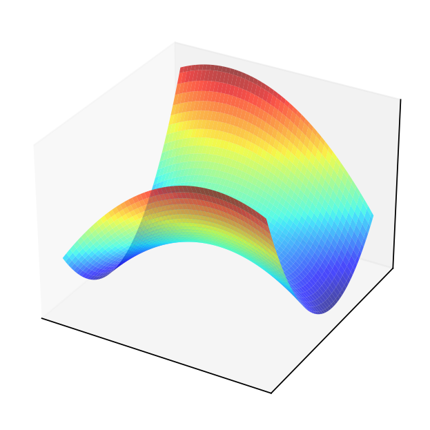
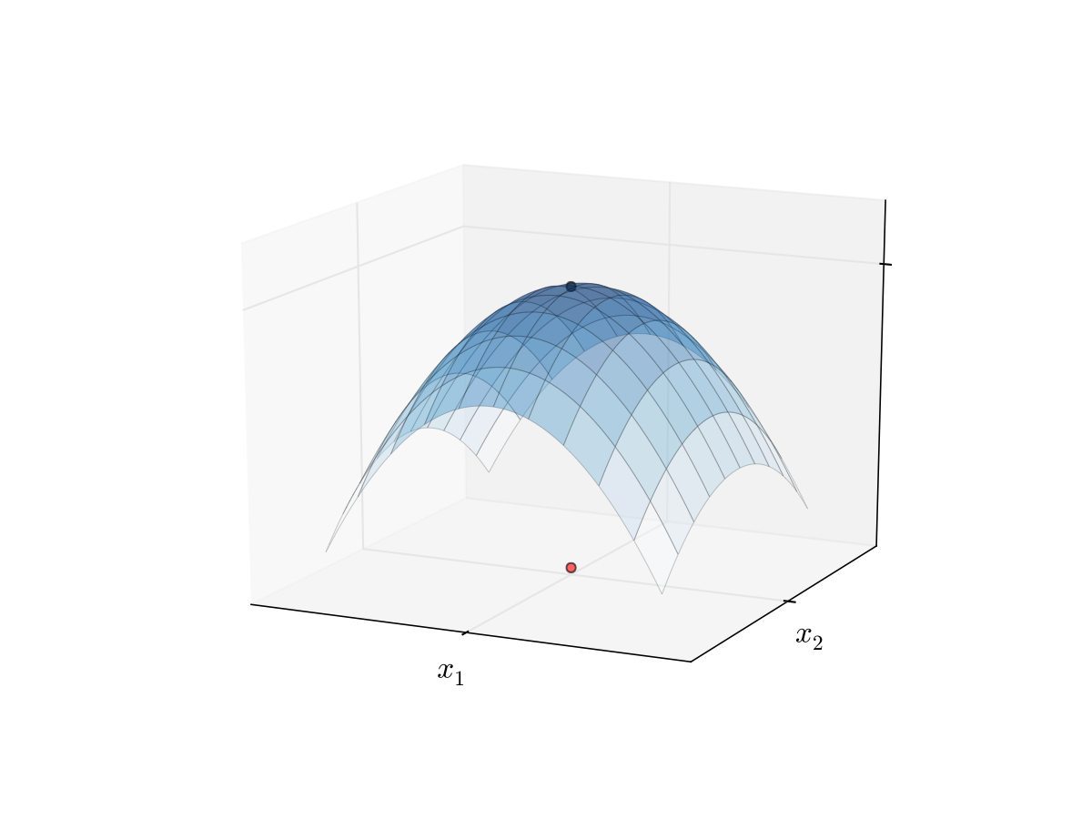
Example

Consider quadratic form \(f({\bf x}) = {\bf x}' A {\bf x}\) where \(A = \left( \begin{array}{rr} 1,& 0.5 \\ 0.5,& -2 \end{array} \right)\)

Solving the FOC

\[ \nabla f({\bf x}) = 2 {\bf x}' A = 0 \implies {\bf x} = {\bf 0} \]

The point \((0,0)\) should be an optimizer?

Show code cell source Hide code cell source

import numpy as np
import matplotlib.pyplot as plt
from mpl_toolkits.mplot3d import Axes3D
from matplotlib import cm

A = np.array([[1,.5],[.5,-2]])
f = lambda x: -(x@A@x)
x = y = np.linspace(-5.0, 5.0, 100)
X, Y = np.meshgrid(x, y)
zs = np.array([f((x,y)) for x,y in zip(np.ravel(X), np.ravel(Y))])
Z = zs.reshape(X.shape)

fig = plt.figure(dpi=160)
ax1 = fig.add_subplot(111, projection='3d')
ax1.plot_surface(X, Y, Z, 
            rstride=2, 
            cstride=2,
            cmap=cm.jet,
            alpha=0.7,
            linewidth=0.25)
plt.setp(ax1,xticks=[],yticks=[],zticks=[])

fig = plt.figure(dpi=160)
ax2 = fig.add_subplot(111)
ax2.set_aspect('equal', 'box')
ax2.contour(X, Y, Z, 50,
            cmap=cm.jet)
plt.setp(ax2, xticks=[],yticks=[])

fig = plt.figure(dpi=160)
ax3 = fig.add_subplot(111, projection='3d')
ax3.plot_wireframe(X, Y, Z, 
            rstride=2, 
            cstride=2,
            alpha=0.7,
            linewidth=0.25)
f0 = f(np.zeros((2)))+0.1
ax3.scatter(0, 0, f0, c='black', marker='o', s=10)
ax3.plot([-3,3],[0,0],[f0,f0],color='black')
ax3.plot([0,0],[-3,3],[f0,f0],color='black')
plt.setp(ax3,xticks=[],yticks=[],zticks=[])

plt.show()

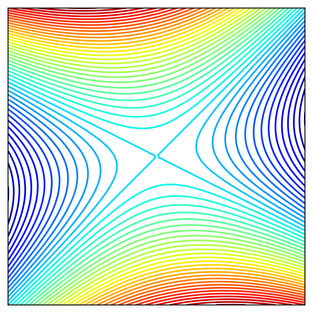
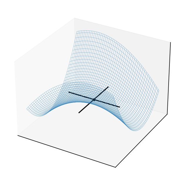
• This is an example of a saddle point where the FOC hold, yet the point is not a local maximizer/minimizer!

• Similar to \(x=0\) in \(f(x) = x^3\): derivative is zero, yet the point is not an optimizer

• How to distinguish saddle points from optima? Key insight: the function has different second order derivatives in different directions!

Second order conditions (SOC)

• allow to establish whether the stationary point is a local maximizer/minimizer or a saddle point

• help to determine whether an optimizer is a maximizer or a minimizer

• do not give definitive answer in all cases, unfortunately

Definition

Let \(A\) be a \(N \times N\) symmetric matrix. It is called

• positive definite if \({\bf x}' {\bf A} {\bf x} > 0\) for all \({\bf x} \in \mathbb{R}^N\) with \({\bf x} \ne {\bf 0}\)

• nonnegative definite (or positive semi-definite) if \({\bf x}' {\bf A} {\bf x} \geq 0\) for all \({\bf x} \in \mathbb{R}^N\)

• negative definite if \({\bf x}' {\bf A} {\bf x} < 0\) for all \({\bf x} \in \mathbb{R}^N\) with \({\bf x} \ne {\bf 0}\)

• nonpositive definite (or negative semi-definite) if \({\bf x}' {\bf A} {\bf x} \leq 0\) for all \({\bf x} \in \mathbb{R}^N\)

Fact (necessary SOC)

Let \(f(x) \colon \mathbb{R}^N \to \mathbb{R}\) be a twice continuously differentiable function and let \({\bf x^\star} \in \mathbb{R}^N\) be a local maximizer/minimizer of \(f\). Then:

• \(f\) has a local maximum at \({\bf x^\star} \implies Hf({\bf x^\star})\) is negative semi-definite

• \(f\) has a local minimum at \({\bf x^\star} \implies Hf({\bf x^\star})\) is positive semi-definite

Fact (sufficient SOC)

Let \(f(x) \colon \mathbb{R}^N \to \mathbb{R}\) be a twice continuously differentiable function. Then:

• if for some \({\bf x^\star} \in \mathbb{R}^N\) \(\nabla f({\bf x^\star}) = {\bf 0}\) (FOC satisfied) and \(Hf({\bf x^\star})\) is negative definite, then \({\bf x^\star}\) is a strict local maximum of \(f\)

• if for some \({\bf x^\star} \in \mathbb{R}^N\) \(\nabla f({\bf x^\star}) = {\bf 0}\) (FOC satisfied) and \(Hf({\bf x^\star})\) is positive definite, then \({\bf x^\star}\) is a strict local minimum of \(f\)

• observe that SOC are only necessary in the “weak” form, but are sufficient in the “strong” form

• this leaves room for ambiguity when we can not arrive at a conclusion — particular stationary point may be a local maximum or minimum

• but we can rule out saddle points for sure, in this case neither semi-definiteness nor definiteness can be established, the Hessian is indefinite

Example

Consider a one dimensional function \(f(x) = (x-1)^2\), \(\nabla f(x)=2x-2\), \(Hf(x) = 2\).

Point \(x=1\) is a stationary point where FOC is satisfied.

Treating \(Hf(x)\) as \(1 \times 1\) matrix, we can see it is positive definite at \(x=1\) (\(y'[2]y = 2y^2 > 0\) for all \(y \ne 0\)), therefore \(x=1\) is a strict local minimum of \(f\).

Example

Consider a one dimensional function \(f(x) = x^2-1\), \(\nabla f(x)=2x\), \(Hf(x) = 2\).

Point \(x=0\) is a stationary point where FOC is satisfied.

Treating \(Hf(x)\) as \(1 \times 1\) matrix, we can see it is positive definite at \(x=0\) (\(y'[2]y = 2y^2 > 0\) for all \(y \ne 0\)), therefore \(x=0\) is a strict local minimum of \(f\).

Example

Consider a one dimensional function \(f(x) = (x-1)^4\), \(\nabla f(x)=4(x-1)^3\), \(Hf(x) = 12(x-1)^2\).

Point \(x=1\) is a stationary point where FOC is satisfied.

Treating \(Hf(x)\) as \(1 \times 1\) matrix, we can see it is positive semi-definite (and negative semi-definite) at \(x=1\) (\(y'[0]y = 0 \ge 0\) and \(y'[0]y = 0 \le 0\) for all \(y \in \mathbb{R}\)), therefore at \(x=1\) function \(f\) may have a local minimum. But may have a local maximum as well. No definite conclusion! (In reality it is a local and global minimum)

Example

Consider a one dimensional function \(f(x) = (x+1)^3\), \(\nabla f(x)=3(x+1)^2\), \(Hf(x) = 6(x+1)\).

Point \(x=-1\) is a stationary point where FOC is satisfied.

Treating \(Hf(x)\) as \(1 \times 1\) matrix, we can see it is positive semi-definite (and negative semi-definite) at \(x=-1\) (\(y'[0]y = 0 \ge 0\) and \(y'[0]y = 0 \le 0\) for all \(y \in \mathbb{R}\)), therefore at \(x=1\) function \(f\) may have a local minimum. But may have a local maximum as well. No definite conclusion! (In reality it is neither local minimum nor maximum)

Establishing definiteness of Hessian in \(\mathbb{R}^2\) case

Recall the following facts from the lecture on linear algebra

Fact

A symmetric matrix \({\bf A}\) is

• positive definite \(\iff\) all eigenvalues are strictly positive

• negative definite \(\iff\) all eigenvalues are strictly negative

• nonpositive definite \(\iff\) all eigenvalues are nonpositive

• nonnegative definite \(\iff\) all eigenvalues are nonnegative

• indefinite \(\iff\) there are both positive and negative eigenvalues

Fact

For any square matrix \({\bf A}\)

\[ % \lambda \text{ is an eigenvalue of } {\bf A} \; \iff \; \det({\bf A} - \lambda {\bf I}) = 0 % \]

Let \(H\) be a \(2 \times 2\) matrix

\[\begin{split} H = \left( \begin{array}{cc} a & b \\ c & d \\ \end{array} \right) \quad \implies \quad H - \lambda {\bf I} = \left( \begin{array}{cc} a - \lambda & b \\ c & d - \lambda \end{array} \right) \end{split}\]

\[\begin{split} \implies \det(H - \lambda {\bf I}) = (a - \lambda)(d - \lambda) - bc \\ = \lambda^2 - (a + d) \lambda + (ad - bc) \\ = \lambda^2 - \mathrm{trace}(H) \lambda + \det(H) \end{split}\]

Hence the the two eigenvalues \(\lambda_1\) and \(\lambda_2\) of \(H\) are given by the two roots of

\[ \lambda^2 - \mathrm{trace}(H) \lambda + \det(H) = 0 \]

From the Viets’s formulas for a quadratic polynomial we have

\[\begin{split} \lambda_1 + \lambda_2 = \mathrm{trace}(H) \\ \lambda_1 \lambda_2 = \mathrm{det}(H) \end{split}\]

Applying this result to a Hessian of a function \(f: \mathbb{R}^2 \to \mathbb{R}\) we have

Fact

Given a twice continuously differentiable function \(f: \mathbb{R}^2 \to \mathbb{R}\) and a stationary point \({\bf x^\star}: \; \nabla f({\bf x^\star}) = {\bf 0}\), the second order conditions provide:

1. if \(\mathrm{det}(Hf({\bf x^\star})) > 0\) and \(\mathrm{trace}(Hf({\bf x^\star})) > 0\) \(\implies\)

   • \(\lambda_1 > 0\) and \(\lambda_2 > 0\),

   • \(Hf({\bf x^\star})\) is positive definite,

   • \(f\) has a strict local minimum at \({\bf x^\star}\)

2. if \(\mathrm{det}(Hf({\bf x^\star})) > 0\) and \(\mathrm{trace}(Hf({\bf x^\star})) < 0\) \(\implies\)

   • \(\lambda_1 < 0\) and \(\lambda_2 < 0\),

   • \(Hf({\bf x^\star})\) is negative definite,

   • \(f\) has a strict local maximum at \({\bf x^\star}\)

3. if \(\mathrm{det}(Hf({\bf x^\star})) = 0\) and \(\mathrm{trace}(Hf({\bf x^\star})) > 0\) \(\implies\)

   • \(\lambda_1 = 0\) and \(\lambda_2 > 0\),

   • \(Hf({\bf x^\star})\) is positive semi-definite (nonnegative definite),

   • \(f\) may have a local minimum \({\bf x^\star}\)

   • undeceive!

4. if \(\mathrm{det}(Hf({\bf x^\star})) = 0\) and \(\mathrm{trace}(Hf({\bf x^\star})) < 0\) \(\implies\)

   • \(\lambda_1 = 0\) and \(\lambda_2 < 0\),

   • \(Hf({\bf x^\star})\) is negative semi-definite (nonpositive definite),

   • \(f\) may have a local maximum \({\bf x^\star}\)

   • undeceive!

5. if \(\mathrm{det}(Hf({\bf x^\star})) < 0\)

   • \(\lambda_1\) and \(\lambda_2\) have different signs,

   • \(Hf({\bf x^\star})\) is indefinite,

   • \({\bf x^\star}\) is a saddle point of \(f\)

Example

Consider a two dimensional function \(f({\bf x}) = (x_1-1)^2 + x_1 x_2^2\)

\[\begin{split} \nabla f({\bf x})=\big( 2(x_1-1) + x_2^2, \; 2 x_1 x_2 \big), \quad Hf({\bf x})= \left( \begin{array}{ll} 2,& 2 x_2 \\ 2 x_2,& 2 x_1 \end{array} \right) \end{split}\]

Point \({\bf x_1^\star}=(1,0)\) is a stationary point where FOC is satisfied.

\[\begin{split} Hf({\bf x^\star}) = \left( \begin{array}{ll} 2,& 0 \\ 0,& 2 \end{array} \right), \quad \mathrm{det}(Hf({\bf x^\star})) = 4 > 0, \quad \mathrm{trace}(Hf({\bf x^\star})) = 4 > 0 \end{split}\]

Therefore at \({\bf x_1^\star}=(1,0)\) function \(f\) has a strict local minimum.

Point \({\bf x_2^\star}=(1+\tfrac{\sqrt{2}}{2},-\sqrt{2})\) is also a stationary point where FOC is satisfied.

\[\begin{split} Hf({\bf x^\star}) = \left( \begin{array}{ll} 2,& 2\sqrt{2} \\ 2\sqrt{2},& 2-\sqrt{2} \end{array} \right), \quad \mathrm{det}(Hf({\bf x^\star})) = -4 - 2\sqrt{2} < 0 \end{split}\]

Therefore at \({\bf x_2^\star}=(1,0)\) function \(f\) has a saddle point.

Point \({\bf x_3^\star}=(1-\tfrac{\sqrt{2}}{2},\sqrt{2})\) is yet another stationary point where FOC is satisfied.

\[\begin{split} Hf({\bf x^\star}) = \left( \begin{array}{ll} 2,& -2\sqrt{2} \\ -2\sqrt{2},& 2+\sqrt{2} \end{array} \right), \quad \mathrm{det}(Hf({\bf x^\star})) = 2\sqrt{2} -4 < 0 \end{split}\]

Therefore again, at \({\bf x_3^\star}=(1,0)\) function \(f\) has a saddle point.

Convexity, sufficiency and uniqueness

A path to globally sufficient conditions for optimality is through establishing the shape of the objective function

• Concave functions \(\rightarrow\) local maxima are global maxima

• Convex functions \(\rightarrow\) local minima are global minima

• Strict concavity/convexity \(\rightarrow\) uniqueness of the maximum/minimum

Convex functions

Definition

\(f \colon A \subset\mathbb{R}^N \to \mathbb{R}\) is called convex if \( f(\lambda {\bf x} + (1 - \lambda) {\bf y}) \leq \lambda f({\bf x}) + (1 - \lambda) f({\bf y}) \) for all \({\bf x}, {\bf y} \in A\) and all \(\lambda \in [0, 1]\)

\(f\) is called strictly convex if \( f(\lambda {\bf x} + (1 - \lambda) {\bf y}) < \lambda f({\bf x}) + (1 - \lambda) f({\bf y}) \) for all \({\bf x}, {\bf y} \in A\) with \({\bf x} \ne {\bf y}\) and all \(\lambda \in (0, 1)\)

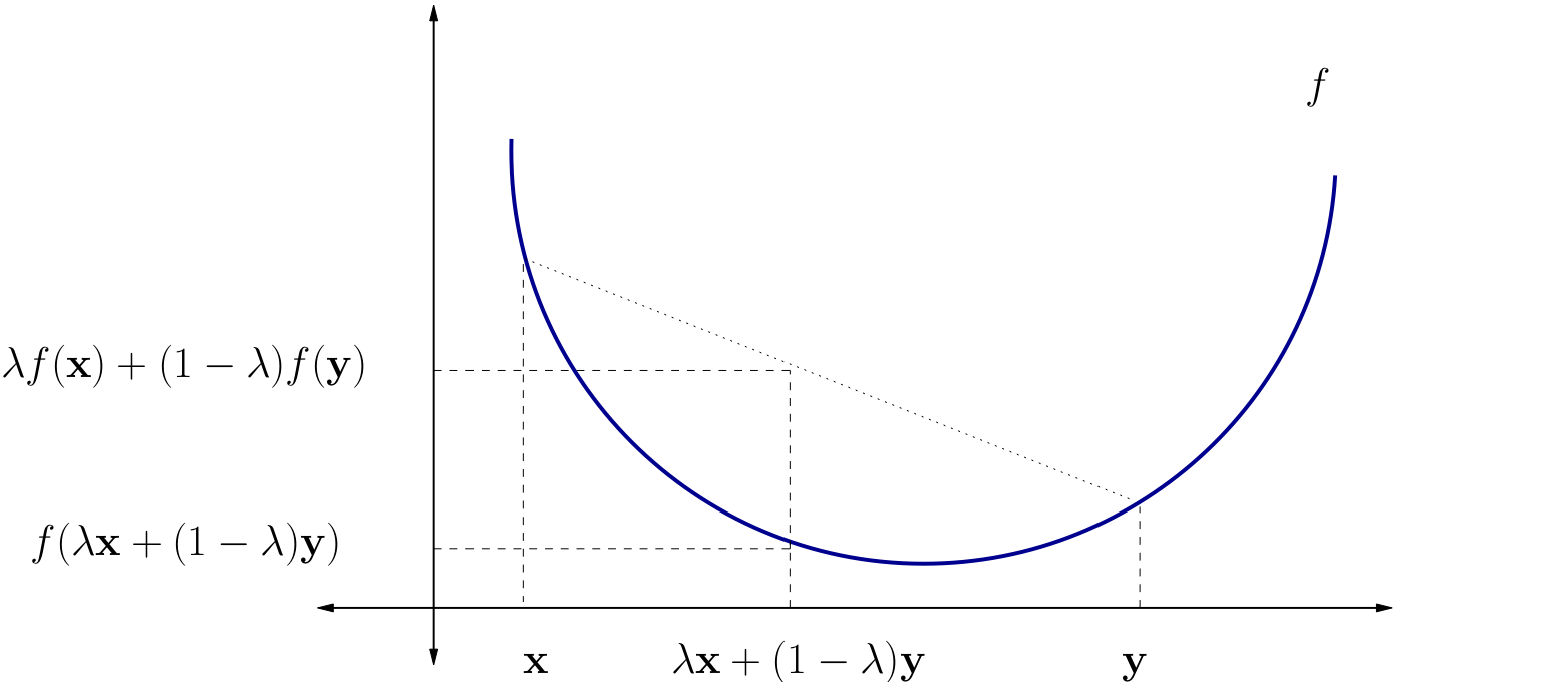
Fig. 84 A strictly convex function on a subset of \(\mathbb{R}\)

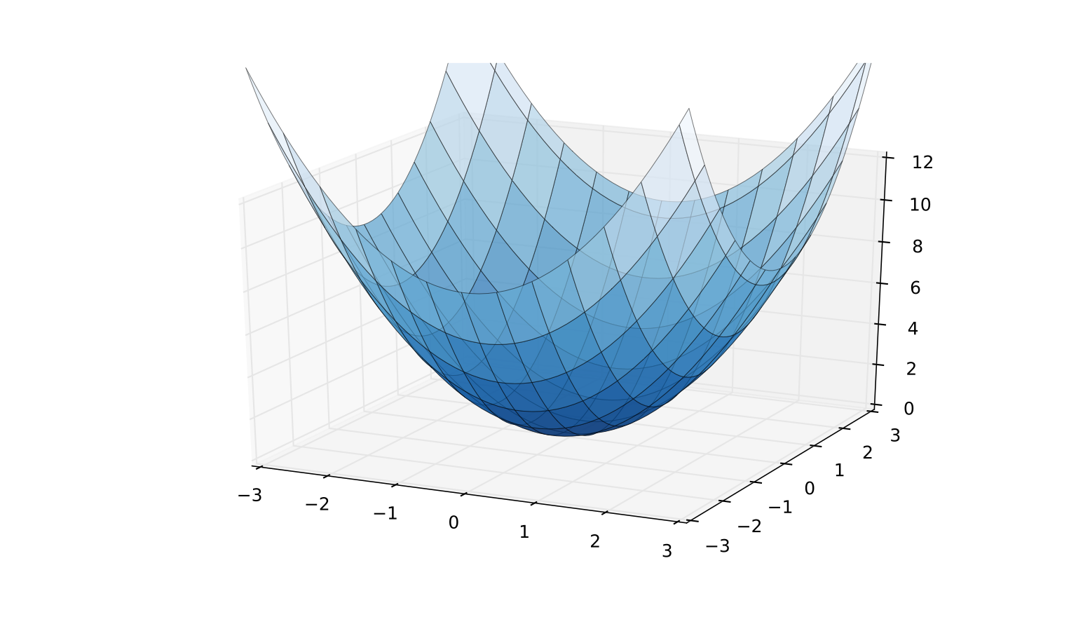
Fig. 85 A strictly convex function on a subset of \(\mathbb{R}^2\)

Example

\(f({\bf x}) = \|{\bf x}\|\) is convex on \(\mathbb{R}^K\)

Proof

To see this recall that, by the properties of norms,

\[\begin{split} \|\lambda {\bf x} + (1 - \lambda) {\bf y}\| \leq \|\lambda {\bf x}\| + \|(1 - \lambda) {\bf y}\| \\ = \lambda \|{\bf x}\| + (1 - \lambda) \|{\bf y}\| \end{split}\]

That is,

\[ % f(\lambda {\bf x} + (1 - \lambda) {\bf y}) \leq \lambda f({\bf x}) + (1 - \lambda) f({\bf y}) % \]

Fact

If \({\bf A}\) is \(K \times K\) and positive definite, then \(Q({\bf x}) = {\bf x}' {\bf A} {\bf x}, {\bf x} \in \mathbb{R}^K\) is strictly convex on \(\mathbb{R}^K\)

Proof

Proof: Fix \({\bf x}, {\bf y} \in \mathbb{R}^K\) with \({\bf x} \ne {\bf y}\) and \(\lambda \in (0, 1)\)

Exercise: Show that

\[\begin{split} % \lambda Q({\bf x}) + (1 - \lambda) Q({\bf y}) - Q(\lambda {\bf x} + (1 - \lambda) {\bf y}) \\ = \lambda (1 - \lambda) ({\bf x} - {\bf y})' {\bf A} ({\bf x} - {\bf y}) % \end{split}\]

Since \({\bf x} - {\bf y} \ne {\bf 0}\) and \(0 < \lambda < 1\), the right hand side is \(> 0\)

Hence

\[ % \lambda Q({\bf x}) + (1 - \lambda) Q({\bf y}) > Q(\lambda {\bf x} + (1 - \lambda) {\bf y}) % \]

Concave Functions

Let \(A \subset \mathbb{R}^K\) be a convex and let \(f\) be a function from \(A\) to \(\mathbb{R}\)

Definition

\(f\) is called concave if

\[ % f(\lambda {\bf x} + (1 - \lambda) {\bf y}) \geq \lambda f({\bf x}) + (1 - \lambda) f({\bf y}) % \]

for all \({\bf x}, {\bf y} \in A\) and all \(\lambda \in [0, 1]\)

\(f\) is called strictly concave if

\[ % f(\lambda {\bf x} + (1 - \lambda) {\bf y}) > \lambda f({\bf x}) + (1 - \lambda) f({\bf y}) % \]

for all \({\bf x}, {\bf y} \in A\) with \({\bf x} \ne {\bf y}\) and all \(\lambda \in (0, 1)\)

Exercise: Show that

1. \(f\) is concave if and only if \(-f\) is convex

2. \(f\) is strictly concave if and only if \(-f\) is strictly convex

Hessian based criterion

Fact

If \(f \colon A \to \mathbb{R}\) is a \(C^2\) function where \(A \subset \mathbb{R}^K\) is open and convex, then

1. \(Hf({\bf x})\) positive semi-definite (nonnegative definite) for all \({\bf x} \in A\) \(\iff f\) convex

2. \(Hf({\bf x})\) negative semi-definite (nonpositive definite) for all \({\bf x} \in A\) \(\iff f\) concave

In addition,

1. \(Hf({\bf x})\) positive definite for all \({\bf x} \in A\) \(\implies f\) strictly convex

2. \(Hf({\bf x})\) negative definite for all \({\bf x} \in A\) \(\implies f\) strictly concave

Proof: Omitted

Example

Let \(A := (0, \infty) \times (0, \infty)\) and let \(U \colon A \to \mathbb{R}\) be the utility function

\[ % U(c_1, c_2) = \alpha \ln c_1 + \beta \ln c_2 % \]

Assume that \(\alpha\) and \(\beta\) are both strictly positive

Exercise: Show that the Hessian at \({\bf c} := (c_1, c_2) \in A\) has the form

\[\begin{split} % H({\bf c}) := \begin{pmatrix} - \frac{\alpha}{c_1^2} & 0 \\ 0 & - \frac{\beta}{c_2^2} \end{pmatrix} % \end{split}\]

Exercise: Show that any diagonal matrix with strictly negative elements along the principle diagonal is negative definite

Conclude that \(U\) is strictly concave on \(A\)

Uniqueness of optimizers

Fact

Let \(A \subset \mathbb{R}^K\) be convex and let \(f \colon A \to \mathbb{R}\)

1. If \(f\) is strictly convex, then \(f\) has at most one minimizer on \(A\)

2. If \(f\) is strictly concave, then \(f\) has at most one maximizer on \(A\)

Interpretation, strictly concave case:

• we don’t know in general if \(f\) has a maximizer

• but if it does, then it has exactly one

• in other words, we have uniqueness

Proof

Proof for the case where \(f\) is strictly concave:

Suppose to the contrary that

• \({\bf a}\) and \({\bf b}\) are distinct points in \(A\)

• both are maximizers of \(f\) on \(A\)

By the def of maximizers, \(f({\bf a}) \geq f({\bf b})\) and \(f({\bf b}) \geq f({\bf a})\)

Hence we have \(f({\bf a}) = f({\bf b})\)

By strict concavity, then

\[ % f\left( \frac{1}{2} {\bf a} + \frac{1}{2} {\bf b} \right) > \frac{1}{2} f( {\bf a}) + \frac{1}{2} f( {\bf b}) = \frac{1}{2} f( {\bf a}) + \frac{1}{2} f( {\bf a}) = f({\bf a}) % \]

This contradicts the assumption that \({\bf a}\) is a maximizer

Fact (sufficient conditions)

If \(f\) and \(A\) are as above and \({\bf x}^* \in A\) is stationary (FOC are satisfied), then

1. \(f\) strictly concave \(\implies\) \({\bf x}^*\) is the unique maximizer of \(f\) on \(A\)

2. \(f\) strictly convex \(\implies\) \({\bf x}^*\) is the unique minimizer of \(f\) on \(A\)

Roadmap for unconstrained optimization

1. Assuming that the domain of the objective function is the whole space, check that it is continuous and for derivative based methods twice continuously differentiable

2. Derive the gradient and Hessian of the objective function. If it can be shown that the function is globally concave or convex, checking SOC (below) is not necessary, and global optima can be established

3. Find all stationary points by solving FOC

4. Check SOC to determine whether found stationary points are (local) maxima or minima and filter out saddle points

5. Assess whether any of the local optima are global by comparing function values at these points, and inspecting the shape of the function to determine if its value anywhere exceeds the best local optimum (limits at the positive and negative infinities, possible vertical asymptotes, etc.)

Extra study material

Note on matrix calculus by Randal J. Barnes, Department of Civil Engineering, University of Minnesota Minneapolis