Exercise set G

Please, see the general comment on the tutorial exercises

Question G.1

Solve the following constrained maximization problem using the Lagrange method, including the second order conditions.

\[\begin{split} % f(x,y) = \frac{x^3}{3}-3y^2+2x \to \max_{x,y} \\ \text {subject to} \\ 4x = y^3,\\ x,y \in \mathbb{R}% \end{split}\]

Hint

1. Write down the Lagrangian function \(\mathcal{L}({\bf x},{\bf \lambda})\)

2. Find all stationary points of \(\mathcal{L}({\bf x},{\bf \lambda})\) with respect to \({\bf x}\) and \({\bf \lambda}\), i.e. solve the system of first order equations

3. Derive the bordered Hessian \(H \mathcal{L}({\bf x},{\bf \lambda})\) and compute it value at the stationary points

4. Using second order conditions, check if the stationary points are local optima

5. Compare the function values at all identified local optima to find the global one

Question G.2

Solve the following constrained maximization problem using the Karush-Kuhn-Tucker method. Verify that the found stationary/critical points satisfy the second order conditions.

\[\begin{split} % f(x,y) = x^3 - y^3 \to \max_{x,y}\\ \text {subject to} \\ x^2 + y^2 \le 1,\\ x,y \in \mathbb{R}% \end{split}\]

Hint

1. Write down the Lagrangian function \(\mathcal{L}({\bf x},{\bf \lambda})\)

2. Solve the KKT first order conditions to find the stationary points of \(\mathcal{L}({\bf x},{\bf \lambda})\) with respect to \({\bf x}\), together with the non-negativity of KKT multipliers and complimentary slackness conditions

3. Using second order conditions using the subset of binding constraints, check if the stationary points at the boundary are local optima. Similarly, using the second order conditions for the unconstrained problem to investigate the interior stationary points

4. Compare the function values at all identified local optima to find the global one

Solutions

Question G.1

Let \(f(x,y)= x^3/3 - 3y^2 + 2x\) and \(g(x,y)=4x-y^3\) for all \(x,y∈\mathbb{R}\). The constraint set is \(\{(x,y): g(x,y)=0\}\). The Lagrangian function is

\[ % \mathcal{L}(x,y,\lambda) = f(x,y) - \lambda g(x,y) = f(x,y)= x^3/3 - 3y^2 + 2x - \lambda(4x-y^3)% \]

The first order partial derivatives are

\[\begin{split} % \frac{\partial \mathcal{L}}{\partial x}= x^2 + 2 - 4 \lambda \\ \frac{\partial \mathcal{L}}{\partial y}= -6y + 3\lambda y^2 \\ \frac{\partial \mathcal{L}}{\partial \lambda}= -(4x -y^3).% \end{split}\]

The bordered Hessian matrix is

\[\begin{split} % H \mathcal{L}(x,y,\lambda)) = \begin{pmatrix} 0 & \frac{\partial^2 \mathcal{L}}{\partial \lambda \partial x} & \frac{\partial^2 \mathcal{L}}{\partial \lambda \partial y}\\ \frac{\partial^2 \mathcal{L}}{\partial \lambda \partial x}& \frac{\partial^2 \mathcal{L}}{\partial x^2} & \frac{\partial^2 \mathcal{L}}{\partial x \partial y} \\ \frac{\partial^2 \mathcal{L}}{\partial \lambda \partial y}& \frac{\partial^2 \mathcal{L}}{\partial y \partial x} & \frac{\partial^2 \mathcal{L}}{\partial y^2} \end{pmatrix} = \begin{pmatrix} 0& -4& 3y^2 \\ -4& 2x & 0\\ 3y^2& 0&-6 + 6 \lambda y \end{pmatrix}.% \end{split}\]

Observe that \(\mathrm{rank}(Dg)) = \mathrm{rank}((-4, 3 y^2)) = 1\) for all \(x,y ∈ \mathbb{R}\). That is, the constrained qualification holds for all points on the constraint.

The first order conditions are

\[\begin{split} % \frac{\partial \mathcal{L}}{\partial x}= x^2 + 2 - 4 \lambda =0\\ \frac{\partial \mathcal{L}}{\partial y}= -6y + 3\lambda y^2 =0\\ \frac{\partial \mathcal{L}}{\partial \lambda}= -(4x -y^3)=0.% \end{split}\]

Observe that if \(\lambda=0\), then the FOCs imply \(x^2+2-4\lambda = x^2+2 = 0\), which is a contradiction since \(x^2+2 ≥ 2\). It must be that \(\lambda ≠ 0\). Next, from the equation \(-6y+3\lambda y^2 = 3y(\lambda y -2)=0\), it is either \(y=0\) or \(y = \lambda/2\).

Case 1: Suppose that \(y=0\). Then, from the constraint \(4x=y^3\) we get \(x=0\). Also, the FOC yields \(x^2+2 - 4\lambda = 0+2-4\lambda=0\) so that \(\lambda=1/2\). Hence, the optimizer is \((x^*, y^*, \lambda^*)=(0,0,1/2)\). The corresponding bordered Hessian matrix is

\[\begin{split} % H\mathcal{L}(0,0,1/2)= \begin{pmatrix} 0 &-4 & 0\\ -4& 0&0\\ 0 &0& -6 \end{pmatrix}% \end{split}\]

Since there are two variables \(N=2\) and one constraint \(K=1\), it suffices to check the last (\(N-K=1\)) leading principal minor, i.e., the determinant of the full bordered Hessian matrix. The determinant follows

\[\begin{split} % \det (H\mathcal{L})=0 - (-4)\begin{vmatrix}-4&0 \\ 0& -6 \end{vmatrix} = 96 >0.% \end{split}\]

It has the same sign as \((-1)^N=(-1)^2\). Therefore, the bordered Hessian matrix is negative definite and \((x^*, y^*, \lambda^*)=(0,0,1/2)\) is a local maximizer on the constraint set.

Case 2: Suppose that \(y=2/\lambda\). Then, by \(\lambda = 2/y\) and \(x = y^3/4\), the FOCs yield

\[\begin{split} % x^2 + 2 - 4 \lambda = y^6/16 + 2 - 8/y = 0 \\ ⇒ y^7 + 32 y - 128=0% \end{split}\]

Let \(h(y)=y^7 + 32 y - 128\). Since \(h'(y)=7 y^6+32 >0\), function \(h\) is strictly increasing. Note that the solution for \(h(y)=0\) is strictly positive since \(y^7\) and \(y\) have the same sign. We can verify that \(y^* ≈ 1.8325\) solves \(h(y)=0\). The optimizer is \((x^*, y^*,\lambda^*)=(\bar{y}^{3}/4, \bar{y}, 2/\bar{y})\) where \(\bar{y}\) satisfies \(h(\bar{y})=0\). The corresponding bordered Hessian is

\[\begin{split} % H\mathcal{L}(\bar{y}^{3}/4, \bar{y}, 2/\bar{y})= \begin{pmatrix} 0& -4& 3 \bar{y}^{2} \\ -4& 2(\bar{y}^{3}/4) & 0\\ 3y^2& 0&-6 + 6 (2/\bar{y}) \bar{y} \end{pmatrix} = \begin{pmatrix} 0& -4& 3 \bar{y}^{2} \\ -4& \bar{y}^{3}/2 & 0\\ 3y^2& 0&6 \end{pmatrix}.% \end{split}\]

The determinant is

\[\begin{split} % \det (H\mathcal{L})= - (-4)\begin{vmatrix}-4& 3\bar{y}^2 \\ 0& 6 \end{vmatrix} +3 \bar{y}^2 \begin{vmatrix}-4& 3\bar{y}^2 \\ \bar{y}^3/2& 0 \end{vmatrix} = -\frac{9}{2}\bar{y}^7 - 96 <0,% \end{split}\]

where the last inequality holds since \(\bar{y}\) is positive. Therefore, \(H\mathcal{L}\) has the same sign as \((-1)^K= -1\) so that it is positive definite. Hence, \((x^*, y^*,\lambda^*)=(\bar{y}^{3}/4, \bar{y}, 2/\bar{y})\) is a local minimizer on the constraint set.

Finally, since \(f(x,y) = x^3/3-3y^2+2x = x^3-3(4x)^{1/3}+2x → \infty\) as \(x→\infty\), there is no global maximizer. The local maximizer on the constraint is \((x,y)=(0,0)\).

Question G.2

The constraint is \(g(x,y) := x^2-y^2 - 1≤ 0\). The Lagrangian function is

\[ \mathcal{L}(x,y,\lambda) = x^3-y^3- \lambda (x^2 + y^2-1)% \]

The necessary KKT conditions are given by the following system of equations and inequalities

\[\begin{split} \frac{\partial \mathcal{L}}{\partial x}= 3x^2 - 2 \lambda x=0\\ \frac{\partial \mathcal{L}}{\partial y}= -3 y^2 -2 \lambda y=0 \\ x^2- y^2-1 \le 0 \\ \lambda ≥ 0 \\ \lambda g(x,y) = \lambda (x^2- y^2-1) = 0% \end{split}\]

To solve this system, we start from checking the two possible cases: \(\lambda=0\) and \(\lambda>0\).

Case 1. \(\lambda=0\): the constraint could not be binding. Then, the FOCs imply \(x=y=0\). The unconstrained Hessian matrix is

\[\begin{split} Hf(0,0) = \begin{pmatrix} \frac{\partial^2 f}{\partial x^2} & \frac{\partial^2 f}{\partial x \partial y} \\ \frac{\partial^2 f}{\partial y \partial x} & \frac{\partial^2 f}{\partial y^2} \end{pmatrix}_{(x,y)=(0,0)} = \begin{pmatrix} 6x & 0\\ 0 & -6y \end{pmatrix}_{(x,y)=(0,0)} = \begin{pmatrix} 0 & 0\\ 0 & 0 \end{pmatrix}_{(x,y)=(0,0)}% \end{split}\]

We have \(\det(H)=0\) and \(trace(H)=0\) so that there is no sufficient information to conclude the property of the stationary point.

Case 2. \(\lambda>0\): the constraint is binding. Then, the problem is the optimization with equality constraint, given two control variables \(N=2\) and one constraint \(K=1\). From the FOCs, we have

\[\begin{split} 0=3x^2 - 2 \lambda x= x(3x -2\lambda) \Longrightarrow x=0, \text{ or } x = \frac{2}{3}\lambda\\ 0=-3 y^2 -2 \lambda y= y(-3y-2\lambda) \Longrightarrow y=0, \text{ or } y = -\frac{2}{3}\lambda\\% \end{split}\]

Since further we have the constraint \(x^2+y^2=1\), there are three cases: “\(x=0, y<0\)”, “\(x>0, y=0\)” or “\(x>0, y<0\)”.

(i) If \(x>0, y<0\), then it follows from the above conditions that

\[\begin{split} \frac{3}{2}x =\lambda = -\frac{3}{2}y \\ ⇒ y=-x.% \end{split}\]

Since \(x^2+y^2=1\) and \(x>0, y<0\), we have \(x=1/\sqrt{2}, y=-1/\sqrt{2}\) and then \(\lambda= 3/(2\sqrt{2})\).

Observe that \(\mathrm{rank}(Dg)) = \mathrm{rank}((2x, 2y)) = 1\) for \(x≠ 0\) or \(y\neq0\), so the constrained qualification holds for any point on the boundary.

The bordered Hessian matrix is

\[\begin{split} H \mathcal{L}(x,y,\lambda)) = \begin{pmatrix} 0 & \frac{\partial^2 \mathcal{L}}{\partial \lambda \partial x} & \frac{\partial^2 \mathcal{L}}{\partial \lambda \partial y}\\ \frac{\partial^2 \mathcal{L}}{\partial \lambda \partial x}& \frac{\partial^2 \mathcal{L}}{\partial x^2} & \frac{\partial^2 \mathcal{L}}{\partial y \partial x} \\ \frac{\partial^2 \mathcal{L}}{\partial \lambda \partial y}& \frac{\partial^2 \mathcal{L}}{\partial x \partial y} & \frac{\partial^2 \mathcal{L}}{\partial y^2} \end{pmatrix} = \begin{pmatrix} 0& -2x& -2y \\ -2x& 6x -2\lambda & 0\\ -2y& 0&-6y -2\lambda \end{pmatrix}.% \end{split}\]

Now, the bordered Hessian at \((x,y,\lambda) = (1/\sqrt{2}, -1/\sqrt{2}, 3/(2\sqrt{2}))\) is

\[\begin{split} H \mathcal{L} (1/\sqrt{2}, -1/\sqrt{2}, 3/(2\sqrt{2}))= \begin{pmatrix} 0& -\sqrt{2}& \sqrt{2} \\ -\sqrt{2}& 3\sqrt{2} -3/\sqrt{2} & 0\\ \sqrt{2}& 0& 3\sqrt{2} -3/\sqrt{2} \end{pmatrix}.% \end{split}\]

It suffices to check the last leading principal minor. The determinant is

\[\begin{split} \begin{align*} \det (H \mathcal{L} (1/\sqrt{2}, -1/\sqrt{2}, 3/(2\sqrt{2})) &= -(-\sqrt{2})\begin{vmatrix} -\sqrt{2}& \sqrt{2} \\ 0& 3\sqrt{2} -3/\sqrt{2} \end{vmatrix} + \sqrt{2}\begin{vmatrix} -\sqrt{2}& \sqrt{2} \\ 3\sqrt{2} -3/\sqrt{2} & 0 \end{vmatrix}\\ &= -6\sqrt{2} < 0, \end{align*}% \end{split}\]

which has the same sign as \((-1)^K=(-1)\). Therefore, it is positive definite and we have a local minimum on the boundary.

(ii) If \(x=0, y<0\), then from \(x^2+y^2=1\), we have \(y=-1\). Also, \(\lambda=-3y/2 = 3/2\). The border Hessian is

\[\begin{split} H \mathcal{L}(0,-1,\frac{3}{2})) = \begin{pmatrix} 0& -2x& -2y \\ -2x& 6x -2\lambda & 0\\ -2y& 0&-6y -2\lambda \end{pmatrix} = \begin{pmatrix} 0&0& 2\\ 0& -3 &0\\ 2&0 & 3 \end{pmatrix}.% \end{split}\]

The determinant is \(\det (H\mathcal{L})=12 >0\), which has the same sign as \((-1)^2\) and then the Hessian matrix is negative definite. Therefore, \((0, -1)\) is a local maximum.

(iii) If \(x>0, y=0\), then from \(x^2+y^2=1\), we have \(x=1\). Also, \(\lambda=3x/2 = 3/2\). The border Hessian is

\[\begin{split} H \mathcal{L}(1,0,\frac{3}{2})) = \begin{pmatrix} 0& -2x& -2y \\ -2x& 6x -2\lambda & 0\\ -2y& 0&-6y -2\lambda \end{pmatrix} = \begin{pmatrix} 0&-2& 0\\ -2& 3 &0\\ 0&0 & -3 \end{pmatrix}.% \end{split}\]

The determinant is \(\det (H\mathcal{L})=12 >0\), which has the same sign as \((-1)^2\) and then the Hessian matrix is negative definite. Therefore, \((1, 0)\) is a local maximum.

Finally, the objective values for the local maximums are \(f(1,0)=f(0,-1)=1\) and note that the constrained set is compact. Therefore, these two local maximizers are also global maximizers.

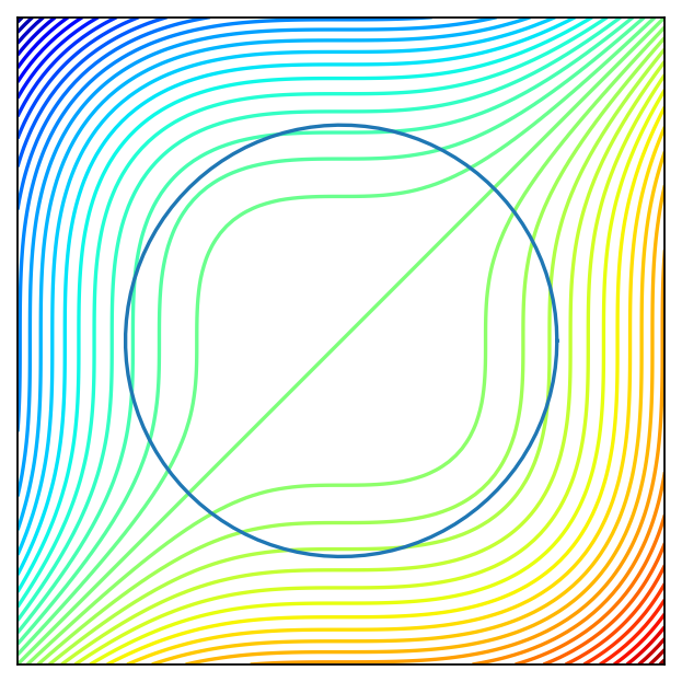
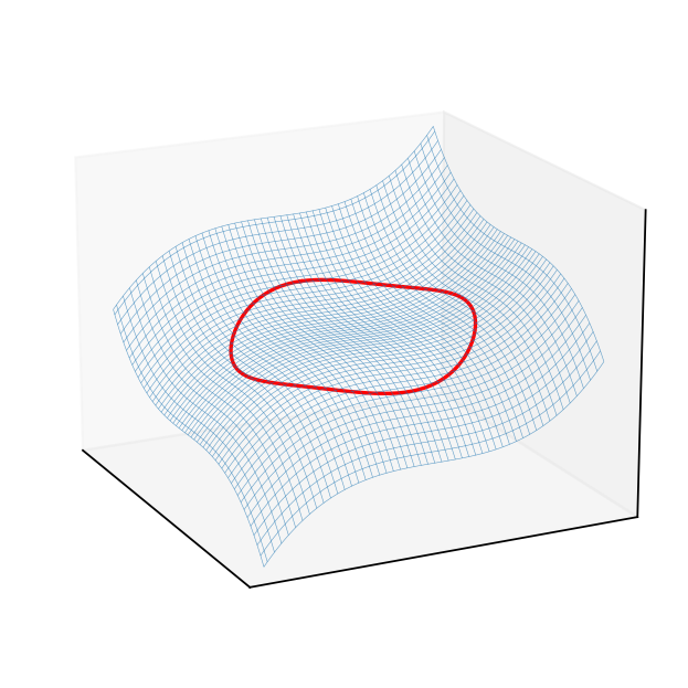
Graphical representation of question G.1

Show code cell source Hide code cell source

import numpy as np
import matplotlib.pyplot as plt
from mpl_toolkits.mplot3d import Axes3D
from matplotlib import cm

f = lambda x: x[0]**3/3 - 3*x[1]**2 + 2*x[0]
gx = lambda y: y**3/4
gy = lambda x: (4*x)**(1/3)

x = y = np.linspace(-5.0, 5.0, 100)
X, Y = np.meshgrid(x, y)
zs = np.array([f((x,y)) for x,y in zip(np.ravel(X), np.ravel(Y))])
Z = zs.reshape(X.shape)

ymax = gy(5.0)
y = np.linspace(-ymax, ymax, 100)
X1,Y1 = gx(y),y
zs = np.array([f((x,y)) for x,y in zip(np.ravel(X1), np.ravel(Y1))])
Z1 = zs.reshape(X1.shape)

fig = plt.figure(dpi=160)
ax1 = fig.add_subplot(111)
ax1.set_aspect('equal', 'box')
ax1.contour(X, Y, Z, 50,
            cmap=cm.jet)
ax1.plot(X1, Y1)
plt.setp(ax1, xticks=[],yticks=[])

fig = plt.figure(dpi=160)
ax2 = fig.add_subplot(111, projection='3d')
ax2.plot_wireframe(X, Y, Z,
            rstride=2,
            cstride=2,
            alpha=0.7,
            linewidth=0.25)
f0 = f(np.zeros((2)))+0.1
ax2.plot(X1, Y1, Z1, c='red')
plt.setp(ax2,xticks=[],yticks=[],zticks=[])
ax2.view_init(elev=18, azim=-160)

plt.show()

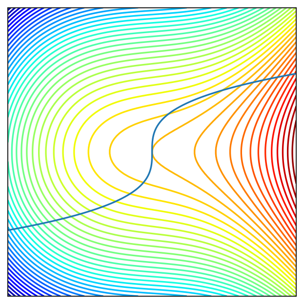
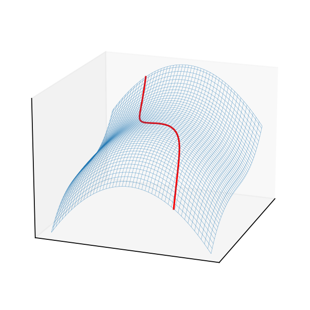
Graphical representation of question G.2

Show code cell source Hide code cell source

import numpy as np
import matplotlib.pyplot as plt
from mpl_toolkits.mplot3d import Axes3D
from matplotlib import cm

f = lambda x: (x[0])**3 - (x[1])**3
lb,ub = -1.5,1.5

x = y = np.linspace(lb,ub, 100)
X, Y = np.meshgrid(x, y)
zs = np.array([f((x,y)) for x,y in zip(np.ravel(X), np.ravel(Y))])
Z = zs.reshape(X.shape)

a,b=1,1
# (x/a)^2 + (y/b)^2 = 1
theta = np.linspace(0, 2 * np.pi, 100)
X1 = a*np.cos(theta)
Y1 = b*np.sin(theta)
zs = np.array([f((x,y)) for x,y in zip(np.ravel(X1), np.ravel(Y1))])
Z1 = zs.reshape(X1.shape)

fig = plt.figure(dpi=160)
ax2 = fig.add_subplot(111)
ax2.set_aspect('equal', 'box')
ax2.contour(X, Y, Z, 50,
            cmap=cm.jet)
ax2.plot(X1, Y1)
plt.setp(ax2, xticks=[],yticks=[])

fig = plt.figure(dpi=160)
ax3 = fig.add_subplot(111, projection='3d')
ax3.plot_wireframe(X, Y, Z,
            rstride=2,
            cstride=2,
            alpha=0.7,
            linewidth=0.25)
f0 = f(np.zeros((2)))+0.1
ax3.plot(X1, Y1, Z1, c='red')
plt.setp(ax3,xticks=[],yticks=[],zticks=[])
ax3.view_init(elev=18, azim=154)

plt.show()