🔬 Tutorial problems lambda

Show code cell content Hide code cell content

import numpy as np
import matplotlib.pyplot as plt
from mpl_toolkits.mplot3d import Axes3D
from matplotlib import cm
from myst_nb import glue

f = lambda x: (x[0])**3 - (x[1])**3
lb,ub = -1.5,1.5

x = y = np.linspace(lb,ub, 100)
X, Y = np.meshgrid(x, y)
zs = np.array([f((x,y)) for x,y in zip(np.ravel(X), np.ravel(Y))])
Z = zs.reshape(X.shape)

a,b=1,1
# (x/a)^2 + (y/b)^2 = 1
theta = np.linspace(0, 2 * np.pi, 100)
X1 = a*np.cos(theta)
Y1 = b*np.sin(theta)
zs = np.array([f((x,y)) for x,y in zip(np.ravel(X1), np.ravel(Y1))])
Z1 = zs.reshape(X1.shape)

fig = plt.figure(dpi=160)
ax2 = fig.add_subplot(111)
ax2.set_aspect('equal', 'box')
ax2.contour(X, Y, Z, 50,
            cmap=cm.jet)
ax2.plot(X1, Y1)
plt.setp(ax2, xticks=[],yticks=[])
glue("pic1", fig, display=False)

fig = plt.figure(dpi=160)
ax3 = fig.add_subplot(111, projection='3d')
ax3.plot_wireframe(X, Y, Z,
            rstride=2,
            cstride=2,
            alpha=0.7,
            linewidth=0.25)
f0 = f(np.zeros((2)))+0.1
ax3.plot(X1, Y1, Z1, c='red')
plt.setp(ax3,xticks=[],yticks=[],zticks=[])
ax3.view_init(elev=18, azim=154)
glue("pic2", fig, display=False)


f = lambda x: x[0]**3/3 - 3*x[1]**2 + 5*x[0] - 6*x[0]*x[1]
x = y = np.linspace(-10.0, 10.0, 100)
X, Y = np.meshgrid(x, y)
zs = np.array([f((x,y)) for x,y in zip(np.ravel(X), np.ravel(Y))])
Z = zs.reshape(X.shape)
a,b=4,8
# (x/a)^2 + (y/b)^2 = 1
theta = np.linspace(0, 2 * np.pi, 100)
X1 = a*np.cos(theta)
Y1 = b*np.sin(theta)
zs = np.array([f((x,y)) for x,y in zip(np.ravel(X1), np.ravel(Y1))])
Z1 = zs.reshape(X1.shape)

fig = plt.figure(dpi=160)
ax2 = fig.add_subplot(111)
ax2.set_aspect('equal', 'box')
ax2.contour(X, Y, Z, 50,
            cmap=cm.jet)
ax2.plot(X1, Y1)
plt.setp(ax2, xticks=[],yticks=[])
glue("pic3", fig, display=False)

fig = plt.figure(dpi=160)
ax3 = fig.add_subplot(111, projection='3d')
ax3.plot_wireframe(X, Y, Z, 
            rstride=2, 
            cstride=2,
            alpha=0.7,
            linewidth=0.25)
f0 = f(np.zeros((2)))+0.1
ax3.plot(X1, Y1, Z1, c='red')
plt.setp(ax3,xticks=[],yticks=[],zticks=[])
ax3.view_init(elev=18, azim=154)
glue("pic4", fig, display=False)

\(\lambda\).1

Formulation

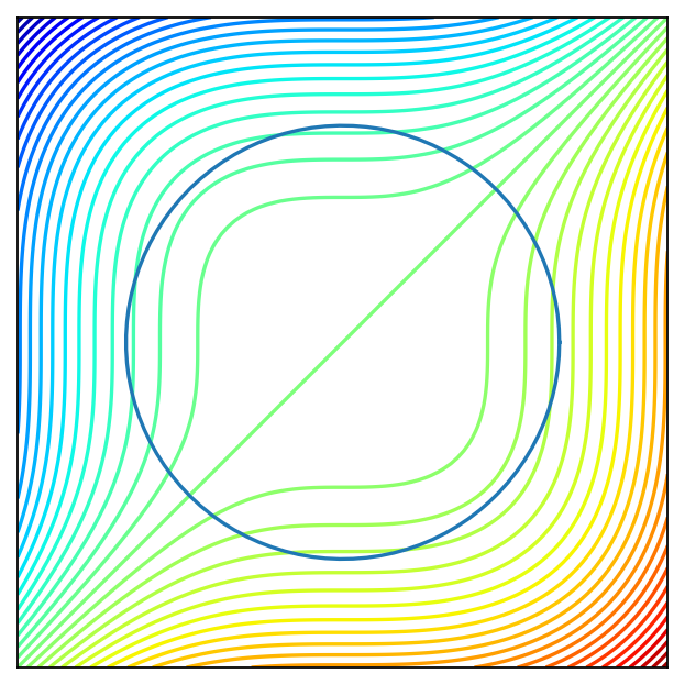
Solve the following constrained maximization problem using the Karush-Kuhn-Tucker method. Verify that the found stationary/critical points satisfy the second order conditions.

\[\begin{split} \begin{array}{c} f(x,y) = x^3 - y^3 \to \max_{x,y}\\ \text {subject to} \\ x^2 + y^2 \le 1,\\ x,y \in \mathbb{R} \end{array} \end{split}\]

Hint

Standard KKT method should work for this problem.

Fig. 100 Level curves of the criterion function and constraint curve.

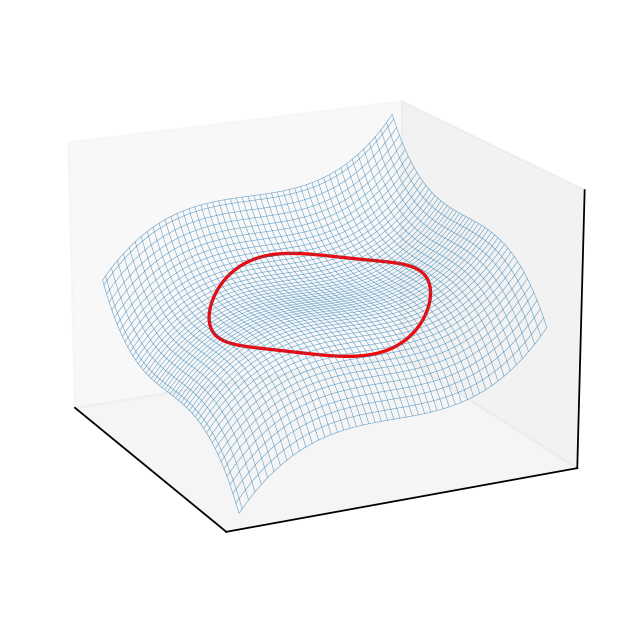
Fig. 101 3D plot of the criterion surface with the constraint curve projected to it.

Solution

⏱

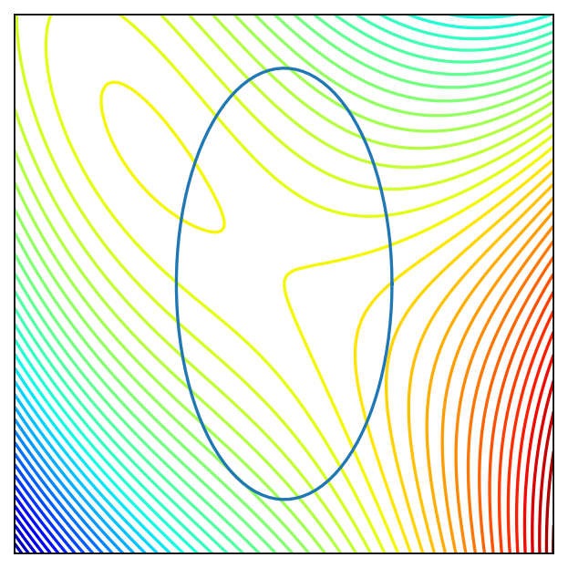
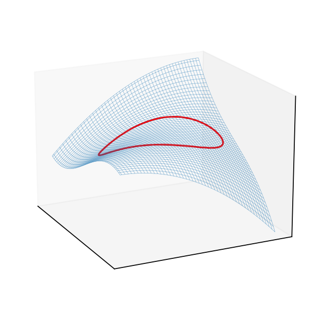
\(\lambda\).2

Formulation

Solve the following constrained maximization problem using the Karush-Kuhn-Tucker method. Verify that the found stationary/critical points satisfy the second order conditions.

\[\begin{split} \begin{array}{c} f(x,y) = -x^2 \to \max_{x,y} \\ \text {subject to} \\ x^2-y^2-2xy \ge 2,\\ x,y \in \mathbb{R} \end{array} \end{split}\]

Hint

Standard KKT method should work for this problem.

Solution

⏱

\(\lambda\).3

Formulation

Roy’s identity

Consider the choice problem of a consumer endowed with strictly concave and differentiable utility function \(u \colon \mathbb{R}^N_{++} \to \mathbb{R}\) where \(\mathbb{R}^N_{++}\) denotes the set of vector in \(\mathbb{R}^N\) with strictly positive elements.

The budget constraint is given by \({\bf p}\cdot{\bf x} \le m\) where \({\bf p} \in \mathbb{R}^N_{++}\) are prices and \(m>0\) is income.

Then the demand function \(x^\star({\bf p},m)\) and the indirect utility function \(v({\bf p},m)\) (value function of the problem) satisfy the equations

\[ x_i^\star({\bf p},m) = -\frac{\partial v}{\partial p_i}({\bf p},m) \Big/ \frac{\partial v}{\partial m}({\bf p},m), \; \forall i \in \{1,\dots,N\} \]

1. Prove the statement

2. Verify the statement by direct calculation (i.e. by expressing the indirect utility and plugging its partials into the identity) using the following specification of utility

\[ u({\bf x}) = \prod_{i=1}^N x_i^{\alpha_i}, \; \alpha_i > 0 \]

Hint

Envelope theorem should be useful here.

Solution

⏱