📖 Sequences, series and convergence

📖 Sequences, series and convergence#

⏱ | words

Sources and reading guide#

Sequences#

Definition

A sequence from a set $X \subset \mathbb{R}$ is a function of the form $f: \mathbb{N} \rightarrow X$.

It is often denoted by $\{ x_n \}^\infty_{n=1}$ or $\{ x_n \}_{n \in \mathbb{N}}$ or $\{ x_1, x_2, \dots , x_n, \dots \}$, where $x_n \in X$ for all $n \in \mathbb{N}$.

In effect, it is indexing of the elements of $X$ by the natural numbers.

Note that this definition of a sequence does not explicitly allow for finite sequences, but we can think about a finite sequence as being a truncated sequence, where we throw away all terms for which $n > N$ for some $N \in \mathbb{N}$. Such a sequence would be written as $\{ x_n \} ^{N}_{n=1}$ or $\{ x_1, x_2, \dots , x_{N} \}$.

Example

$\{x_n\} = \{2, 4, 6, \ldots \}$
$\{x_n\} = \{1, 1/2, 1/4, \ldots \}$
$\{x_n\} = \{1, -1, 1, -1, \ldots \}$
$\{x_n\} = \{0, 0, 0, \ldots \}$

Important notational comment

We have been looking at sequences drawn from some set $X$. The $n$-th element of such a sequence was denoted by $x_n$. This requires that $x_n \in X$.

Do not confuse this $x_n$ with the $n$-th coordinate of the point $x = (x_1, x_2, \dots , x_{(n−1)}, x_n, x_{(n+1)}, \dots , x_L) \in \mathbb{R}^L$.

If we are considering sequences of points (or vectors) in $\mathbb{R}^L$, then we might want to use superscripts to denote sequence position and subscripts to denote coordinates.

In this way, the $k$-th element of the sequence $\{ x_n \}^\infty_{n=1}$ would be the point (or vector) $x_k = (x^k_1, x^k_2, \dots , x^k_{(n−1)}, x^k_n, x^k_{(n+1)}, \dots , x^k_L)$. Note that the $k$ in this case is an index, NOT a power.

Convergence and limit#

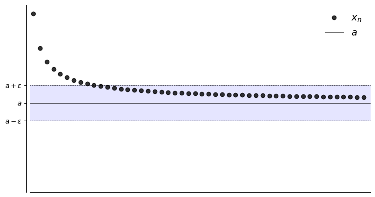
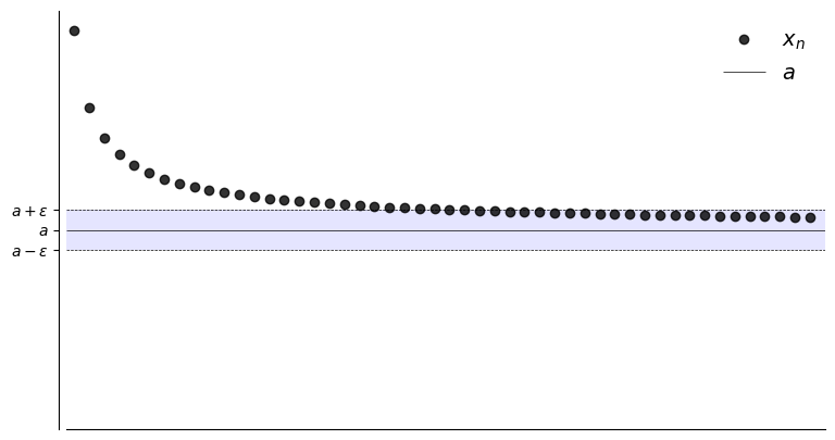
Let $a \in \mathbb{R}$ and let $\{x_n\}$ be a sequence

Suppose, for any $\epsilon > 0$, we can find an $N \in \mathbb{N}$ such that

\[| x_n -a | <\epsilon \text{ for all } n \geq N\]

Then $\{x_n\}$ is said to converge to $a$

Convergence to $a$ in symbols,

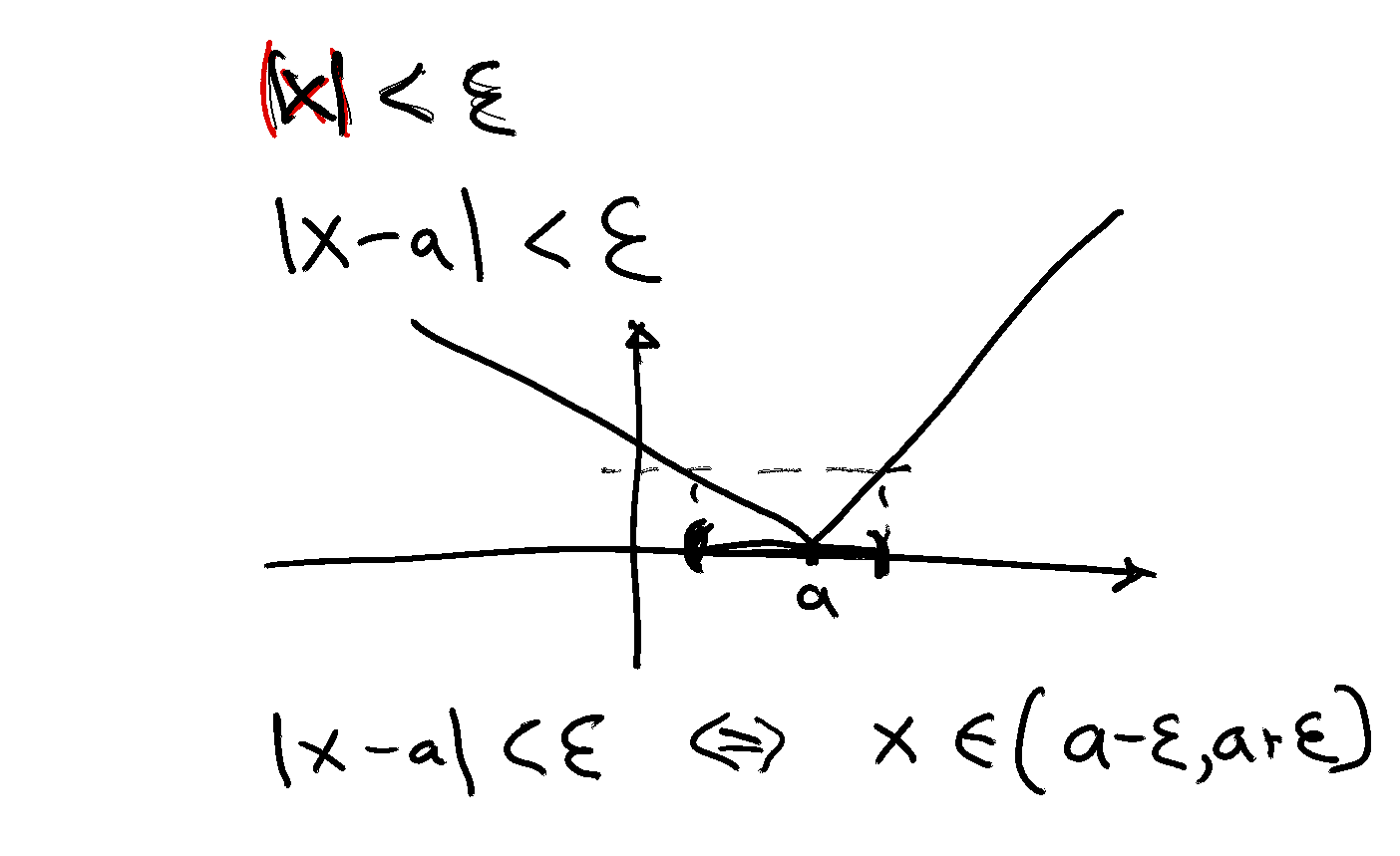
\[\forall \, \epsilon > 0, \; \exists \, N \in \mathbb{N} \; \text{ such that } n \geq N \implies | x_n -a | <\epsilon\]

expression $| x_n -a | <\epsilon$ defines an $\epsilon$-neighborhood around $a$

The sequence $\{x_n\}$ is eventually in this $\epsilon$-neighborhood around $a$

_images/8ddb450b5347850858825e19138e3fe8b2ef5247d4d8807d5c38fbf628d1a613.png

_images/ed9fa35fc5aa4ba73d0e0d617ef78fe9d1c8b0cd3f8e270ed1d597cb5d11bc58.png

_images/b5f50a2f18071cb6badeb05716ecbff61c62a2e036bb8521979a107f8b4ade36.png

Definition

The point $a$ is called the limit of the sequence, denoted

\[x_n \to a \text{ as } n \to \infty \quad \text{ or } \quad \lim_{n \to \infty} x_n = a,\]

if

\[\forall \, \epsilon > 0, \; \exists \, N \in \mathbb{N} \; \text{ such that } n \geq N \implies |x_n - a|< \epsilon\]

Example

$\{x_n\}$ defined by $x_n = 1 + 1/n$ converges to $1$:

\[x_n \to 1 \; \mathrm{as} \; n \to \infty \quad\text{or}\quad \lim_{n \to \infty} x_n = 1\]

To prove this we must show that $\forall \, \epsilon > 0$, there is an $N \in \mathbb{N}$ such that

\[n \geq N \implies |x_n - 1| < \epsilon\]

To show this formally we need to come up with an “algorithm”

You give me any $\epsilon > 0$
I respond with an $N$ such that equation above holds

In general, as $\epsilon$ shrinks, $N$ will have to grow

Proof:

Here’s how to do this for the case $1 + 1/n$ converges to $1$

First pick an arbitrary $\epsilon > 0$

Now we have to come up with an $N$ such that

\[n \geq N \implies |1 + 1/n - 1| < \epsilon\]

Let $N$ be the first integer greater than $ 1/\epsilon$

Then

\[n \geq N \implies n > 1/\epsilon \implies 1/n < \epsilon \implies |1 + 1/n - 1| < \epsilon \]

Remark: Any $N' > N$ would also work

Example

The sequence $x_n = 2^{-n}$ converges to $0$ as $n \to \infty$

Proof:

Must show that, $\forall \, \epsilon > 0$, $\exists \, N \in \mathbb{N}$ such that

\[n \geq N \implies |2^{-n} - 0| < \epsilon\]

So pick any $\epsilon > 0$, and observe that

\[|2^{-n} - 0| < \epsilon \; \iff \; 2^{-n} < \epsilon \; \iff \; n > - \frac{\ln \epsilon}{\ln 2}\]

Hence we take $N$ to be the first integer greater than $- \ln \epsilon / \ln 2$

Then

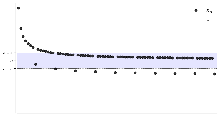
\[n \geq N \implies n > -\frac{\ln \epsilon}{\ln 2} \implies |2^{-n} - 0| < \epsilon\]

What if we want to show that $x_n \to a$ fails?

To show convergence fails we need to show the negation of

\[\forall \,\; \epsilon > 0, \;\; \exists \,\; N \in \mathbb{N} \;\mathrm{such\;that}\; n \geq N \implies |x_n -a|<\epsilon\]

In words, there is an $\epsilon > 0$ where we can’t find any such $N$

That is, for any choice of $N$ there will be $n>N$ such that $x_n$ jumps to the outside $\epsilon$-neighborhood around $a$

In other words, there exists a $\epsilon$ such that $|x_n-a| \geqslant \epsilon$ again and again as $n \to \infty$.

This is the kind of picture we’re thinking of

_images/53d1919304d7ad89f073dba8b2cd3f8bd1d3bfa78a7dba37fed4c2b650b1a5df.png

Example

The sequence $x_n = (-1)^n$ does not converge to any $a \in \mathbb{R}$

Proof:

This is what we want to show

\[\exists \,\; \epsilon > 0 \;\text{ such that } |x_n-a| \geqslant \epsilon \text{ infinitely many times as } n \to \infty\]

Since it’s a “there exists”, we need to come up with such an $\epsilon$

Let’s try $\epsilon = 0.5$, so that the $\epsilon$-neighborhood around $a$ is

\[\{ x \in \mathbb{R} : |x - a| < 0.5 \} = (a-0.5, a+0.5 )\]

We have:

If $n$ is odd then $x_n = -1$ when $n > N$ for any $N$.
If $n$ is even then $x_n = 1$ when $n > N$ for any $N$.

Therefore even if $a=1$ or $a=-1$, $\{x_n\}$ is not in $(a-0.5, a+0.5 )$ infinitely many times as $n \to \infty$.

It holds for all other values of $a \in \mathbb{R}$ as well

Properties of limits#

Fact

$x_n \to a$ in $\mathbb{R}$ if and only if $|x_n - a| \to 0$ in $\mathbb{R}$
If $x_n \to x$ and $y_n \to y$ then $x_n + y_n \to x + y$
If $x_n \to x$ and $\alpha \in \mathbb{R}$ then $\alpha x_n \to \alpha x$
If $x_n \to x$ and $y_n \to y$ then $x_n y_n \to xy$
If $x_n \to x$ and $y_n \to y$ then $x_n / y_n \to x/y$, provided $y_n \ne 0$, $y \ne 0$
If $x_n \to x$ then $x_n^p \to x^p$

Proof

Let’s prove that

\[x_n \to a \; \iff \; |x_n - a| \to 0\]

$x_n \to a$ in $\mathbb{R}$ means that

\[\forall \, \epsilon > 0, \; \exists \, N \in \mathbb{N} \; \mathrm{such\;that} \; n \geq N \implies | x_n - a | < \epsilon\]

$|x_n - a| \to 0$ in $\mathbb{R}$ means that

\[\forall\, \epsilon > 0, \; \exists \, N \in \mathbb{N} \; \mathrm{such\;that} \; n \geq N \implies | | x_n - a | - 0 | < \epsilon\]

Obviously equivalent

Exercise: Prove other properties using definition of limit

Fact

Each sequence in $\mathbb{R}$ has at most one limit

Proof

Proof for the $\mathbb{R}$ case.

Suppose instead that $x_n \to a \text{ and } x_n \to b \text{ with } a \ne b $

Take disjoint $\epsilon$-neighborhoods around $a$ and $b$ as shown

Since $x_n \to a$ and $x_n \to b$,

$\exists \; N_a$ s.t. $n \geq N_a \implies |x_n -a|<\epsilon$
$\exists \; N_b$ s.t. $n \geq N_b \implies |x_n -b|<\epsilon$

But then $n \geq \max\{N_a, N_b\} \implies $ $|x_n -a|<\epsilon$ and $|x_n -b|<\epsilon$

Contradiction, as the intervals around $a$ and $b$ are assumed disjoint

Cauchy sequences#

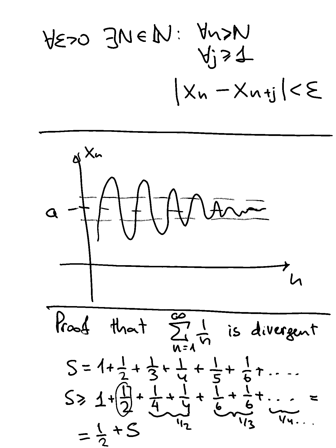
Informal definition: Cauchy sequences are those where $|x_n - x_{n+1}|$ gets smaller and smaller

Example

Sequences generated by iterative methods for solving nonlinear equations often have this property

See code example

Definition

A sequence $\{x_n\}$ is called Cauchy if

\[\forall \; \epsilon > 0, \;\; \exists \; N \in \mathbb{N} \; \mathrm{such\;that}\; \forall n, m \geqslant N \implies | x_n - x_m | < \epsilon\]

Alternatively

\[\forall \; \epsilon > 0, \;\; \exists \; N \in \mathbb{N} \; \mathrm{such\;that}\; \forall j \geqslant N \implies | x_n - x_{n+j} | < \epsilon\]

Cauchy sequences allow to establish convergence without finding the limit itself!

Fact

Every convergent sequence is Cauchy, and every Cauchy sequence is convergent.

Proof

Proof of $\Rightarrow$:

Let $\{x_n\}$ be a sequence converging to some $a \in \mathbb{R}$

Fix $\epsilon > 0$

We can choose $N$ s.t.

\[n \geq N \;\; \implies \;\; |x_n - a | < \frac{\epsilon}{2} \]

For this $N$ we have $n \geq N$ and $j \geq 1$ implies

\[|x_n - x_{n+j}| \leq |x_n - a| + |x_{n+j} - a| < \frac{\epsilon}{2} + \frac{\epsilon}{2} = \epsilon\]

Proof of $\Leftarrow$:

Follows from the density property of $\mathbb{R}$

Example

$\{x_n\}$ defined by $x_n = \alpha^n$ where $\alpha \in (0, 1)$ is Cauchy

Proof:

For any $n , j$ we have

\[|x_n - x_{n+j}| = |\alpha^n - \alpha^{n+j}| = \alpha^n |1 - \alpha^j| \leq \alpha^n\]

Fix $\epsilon > 0$

We can show that $n > \log(\epsilon) / \log(\alpha) \implies \alpha^n < \epsilon$

Hence any integer $N > \log(\epsilon) / \log(\alpha)$ the sequence is Cauchy by definition.

Sub-sequences#

Let $g: \mathbb{N} \rightarrow \mathbb{N}$ be an increasing mapping of the form $g(k) = n_k$.

This means that $g(k + 1) = n_{k+1} > n_k = g(k)$ for all $k \in \mathbb{N}$.

The mapping $f: \mathbb{N} \rightarrow X$ is a sequence from $X$, and so is the mapping $h: \mathbb{N} \rightarrow X$ given by $h = f \circ g$!

Note that $h(k) = f(g(k)) = f(n_k)$.
$f$ generates the sequence $\{x_1, x_2, \dots , x_{n_1 − 1}, x_{n_1} , x_{n_1 + 1}, \dots , x_{n_2 − 1}, x_{n_2}, x_{n_2 + 1}, \dots \}$
$h$ generates the sequence $\{x_{n_1} , x_{n_2} , \dots \}$

Definition

The sequence $\{x_{n_k} \}_{n_k \in \mathbb{N}}$ where $k \in \mathbb{N}$ and $n_{k+1} > n_k$ for all $k$, is referred to as a sub-sequence of the sequence $\{ x_n \}_{n \in \mathbb{N}}$

Note that every term in the sequence $\{ x_{n_k} \}_{n_k \in \mathbb{N}}$ is found somewhere in the sequence $\{ x_n \}_{n \in \mathbb{N}}$

Note also that the (relative) order in which the terms appear is the same for each of the sequences (due to the fact that $n_{k+1} > n_k$ for all $k$)

Example

Consider the sequence $\{ x_n \}_{n \in \mathbb{N}}$ where $x_n = \frac{1}{n}$.

The mapping for this sequence is $f(n) = \frac{1}{n}$.
The sequence looks like $\left\{1, \frac{1}{2}, \frac{1}{3} , \dots , \frac{1}{n}, \dots \right\}$.

Consider the increasing mapping $g: \mathbb{N} \rightarrow \mathbb{N}$ defined by $g(k) = k^2$.

This, along with $f$, generates the sub-sequence mapping

\[ h(k) = f(g(k)) = f(k^2) = \frac{1}{k^2}\]

The associated sub-sequence is

\[ \left\{ \frac{1}{k^2} \right\}_{k \in \mathbb{N}} = \left\{ 1, \frac{1}{4}, \frac{1}{9}, \dots , \frac{1}{n^2} , \dots \right\}\]

Consider the increasing map $g: \mathbb{N} \rightarrow \mathbb{N}$ defined by $g(k) = 2^k$.

This, along with $f$, generates the sub-sequence map

\[h(k) = f(g(k)) = f(2^k) = \frac{1}{2^k}\]

The associated sub-sequence is

\[\left\{ \frac{1}{2^k} \right\}_{k \in \mathbb{N}} = \left\{ \frac{1}{2}, \frac{1}{4}, \frac{1}{8} , \dots , \frac{1}{2^n}, \dots \right\} \]

Fact

If $\{ x_n \}$ converges to $x$ in $\mathbb{R}$, then every subsequence of $\{x_n\}$ also converges to $x$

Fact

If two different subsequences of a sequence converge to different limits, the original sequence is not convergent.

Example

The sequence $\left\{ \frac{1}{n} \right\}_{n \in \mathbb{N}}$ converges to the point $x = 0$.
The sequence $\left\{ \frac{1}{n^2} \right\}_{n \in \mathbb{N}}$ converges to the point $x = 0$.
- Recall that $\left\{ \frac{1}{n^2} \right\}_{n \in \mathbb{N}}$ is a sub-sequence of $\left\{ \frac{1}{n} \right\}_{n \in \mathbb{N}}$
The sequence $\left\{ \frac{1}{2^n} \right\}_{n \in \mathbb{N}}$ converges to the point $x = 0$.
- Recall that $\left\{ \frac{1}{2^n} \right\}_{n \in \mathbb{N}}$ is a sub-sequence of $\left\{ \frac{1}{n} \right\}_{n \in \mathbb{N}}$
The sequence $\left\{ \frac{(−1)^n}{n} \right\}_{n \in \mathbb{N}} = \{ −1, \frac{1}{2}, \frac{−1}{3} , \dots \}$ converges to the point $x = 0$.
The sequence $\left\{ \frac{n}{n + 1} \right\}_{n \in \mathbb{N}} = \{ \frac{1}{2}, \frac{2}{3}, \frac{3}{4}, \dots \}$ converges to the point $x = 1$.
The sequence $\{ (−1)^n \}_{n \in \mathbb{N}} = \{ −1, 1, −1, 1, \dots \}$ does not converge.
The sequence $\{ n \}_{n \in \mathbb{N}}$ does not converge.
The sequence $\left\{ ( \frac{1}{n} , \frac{(n−1)}{n} ) \right\}_{n \in \mathbb{N}}$ converges to $(0, 1)$.
The sequence $\left\{ ( \frac{(−1)^n}{n}, \frac{(−1)^n}{n} ) \right\}_{n \in \mathbb{N}}$ converges to $(0, 0)$.
The sequence $\{ ((−1)^n, (−1)^n) \}_{n \in \mathbb{N}}$ does not converge.
The sequence $\{ (n, n) \}_{n \in \mathbb{N}}$ does not converge.

Mathematical application: Euler’s constant ($e$)#

Euler’s constant, which is usually denoted by $e$, is an irrational number that is defined as the limit of a particular sequence of rational numbers.

Consider the sequence

\[ \{ x_n \}_{n \in \mathbb{N}} = \left\{ \left(1 + \frac{1}{n} \right)^n \right\}_{n \in \mathbb{N}} \]

This sequence converges to Euler’s constant. Euler’s constant is defined to be

\[ e = \lim_{n \rightarrow \infty} \left(1 + \frac{1}{n} \right)^n \]

Computing Euler’s constant as a limit of a sequence

e0 = 2.71828182845904523536028747135266
f = lambda n: (1+1/n)**n
print('Approximation of Euler constant')
for i in range(0,10100,500):
    e = f(i+1)
    print('iter = {:5d}: e = {:14.8f} err = {:14.10f}'.format(i,e,e0-e))

Approximation of Euler constant
iter =     0: e =     2.00000000 err =   0.7182818285
iter =   500: e =     2.71557393 err =   0.0027079019
iter =  1000: e =     2.71692529 err =   0.0013565409
iter =  1500: e =     2.71737689 err =   0.0009049376
iter =  2000: e =     2.71760291 err =   0.0006789198
iter =  2500: e =     2.71773859 err =   0.0005432399
iter =  3000: e =     2.71782907 err =   0.0004527577
iter =  3500: e =     2.71789372 err =   0.0003881134
iter =  4000: e =     2.71794221 err =   0.0003396225
iter =  4500: e =     2.71797993 err =   0.0003019027
iter =  5000: e =     2.71801010 err =   0.0002717240
iter =  5500: e =     2.71803480 err =   0.0002470304
iter =  6000: e =     2.71805538 err =   0.0002264511
iter =  6500: e =     2.71807279 err =   0.0002090370
iter =  7000: e =     2.71808772 err =   0.0001941098
iter =  7500: e =     2.71810066 err =   0.0001811725
iter =  8000: e =     2.71811198 err =   0.0001698519
iter =  8500: e =     2.71812197 err =   0.0001598629
iter =  9000: e =     2.71813084 err =   0.0001509835
iter =  9500: e =     2.71813879 err =   0.0001430386
iter = 10000: e =     2.71814594 err =   0.0001358880

See an excellent video about the Euler constant by Numberphile YouTube

Series#

Definition

A infinite series is the sum of the infinite terms of a sequence $\{ x_n \}_{n \in \mathbb{N}}$ and is denoted by

\[ \sum_{n \in \mathbb{N}} x_n = \sum_{n=1}^{\infty} x_n = x_1 + x_2 + x_3 + \dots \]

Definition

A partial sum of a series is the sum of the first $N$ terms of the sequence,

\[s_N = \sum_{n=1}^{N} x_n = x_1 + x_2 + x_3 + \dots + x_N\]

Definition

The value of the series is equal to the limit of the sequence of its partial sums, when it exists

\[\sum_{n \in \mathbb{N}} x_n = \lim_{N \to \infty} s_N = \lim_{N \to \infty} \sum_{n=1}^{N} x_n\]

If the limit does not exist, the series is referred to as divergent.

We might sometimes want to start the summation at $n = 0$. We can do this by employing a change of index.

If we let $k = n − 1$, the total sum of the sequence can be expressed as

\[ \sum_{n=1}^{\infty} x_n = \sum_{k=0}^{\infty−1} x_{k+1} = \sum_{k=0}^{\infty} x_{k+1}\]

(because $\infty − 1 = \infty$).

If we let $k = n − 1$, the partial sum of the first $N$ terms of the sequence can be expressed as

\[\sum_{n=1}^{N} x_n = \sum_{k=0}^{N - 1} x_{k+1}\]

Example

Euler constant $e$ can be expressed as a series

\[e = \sum_{n=0}^{\infty} \frac{1}{n!} = 1 + 1 + \frac{1}{2} + \frac{1}{6} + \frac{1}{24} + \dots\]

See explanation and derivation in a video

Computing Euler’s constant as series

e0 = 2.71828182845904523536028747135266
print('Approximation of Euler constant with a series')
e = 0.
for n in range(0,21):
    term = term / n if n>0 else 1.
    e += term
    print('iter = {:3d}: e = {:17.15f} err = {:14.7e}'.format(n,e,e0-e))

Approximation of Euler constant with a series
iter =   0: e = 1.000000000000000 err =  1.7182818e+00
iter =   1: e = 2.000000000000000 err =  7.1828183e-01
iter =   2: e = 2.500000000000000 err =  2.1828183e-01
iter =   3: e = 2.666666666666667 err =  5.1615162e-02
iter =   4: e = 2.708333333333333 err =  9.9484951e-03
iter =   5: e = 2.716666666666666 err =  1.6151618e-03
iter =   6: e = 2.718055555555555 err =  2.2627290e-04
iter =   7: e = 2.718253968253968 err =  2.7860205e-05
iter =   8: e = 2.718278769841270 err =  3.0586178e-06
iter =   9: e = 2.718281525573192 err =  3.0288585e-07
iter =  10: e = 2.718281801146385 err =  2.7312661e-08
iter =  11: e = 2.718281826198493 err =  2.2605522e-09
iter =  12: e = 2.718281828286169 err =  1.7287638e-10
iter =  13: e = 2.718281828446759 err =  1.2285728e-11
iter =  14: e = 2.718281828458230 err =  8.1490370e-13
iter =  15: e = 2.718281828458995 err =  5.0182081e-14
iter =  16: e = 2.718281828459043 err =  2.2204460e-15
iter =  17: e = 2.718281828459046 err = -4.4408921e-16
iter =  18: e = 2.718281828459046 err = -4.4408921e-16
iter =  19: e = 2.718281828459046 err = -4.4408921e-16
iter =  20: e = 2.718281828459046 err = -4.4408921e-16

Example

Harmonic series given by

\[\sum_{n=0}^{\infty} \frac{1}{n} = 1 + \frac{1}{2} + \frac{1}{3} + \frac{1}{4} + \dots\]

is divergent. The $n$-th partial sum is approximately equal $\ln(n)+\gamma$, where $\gamma = 0.577$ is called an Euler-Mascheroni constant.

Proof by mathematical induction#

Suppose that we have a series of statements that can be indexed by the set of natural numbers ($\mathbb{N} = \{ 1, 2, \dots , n, \dots \}$) and we want to prove that these statements are true for all $n \in \mathbb{N}$. Denote the $n$-th statement as a claim by $A_n$.

A proof of the claim by deduction might proceed as follows (where the symbol “$\land$” can be interpreted as meaning “and”):

\[ A_1 \land A_2 \land A_3 \dots \land A_n \land \dots \Rightarrow A\]

The (countably) infinite number of cases that would need to be verified for such a proof by deduction to be implemented make it unfeasible. Instead, a proof by induction might be appropriate in such cases.

A proof proceeds as follows:

\[A_1\; \text{ and }\; (\forall n \; A_n \Rightarrow A_{(n+1)}) \Rightarrow A\]

Step 1: Show that the claim is true when $n = 1$.
Step 2: Assume that the claim is true for the arbitrary case of $n = k$ (this is known as the inductive assumption) and show that, if this inductive assumption is true, then the claim must also be true for the case of $n = k + 1$.
Step 3: Apply the principle of mathematical induction to conclude that the claim is true for all $n \in \mathbb{N}$.

The logic underlying a proof by induction is very intuitive. It basically establishes that the claim is true for $n = 1$, and that if the claim is true for $n = 1$, then it must also be true for $n = 2$, which means it must also be true for $n = 3$, which means it must also be true for $n = 4$, and so on and so forth, ad infinitum.

Example

We want to show that $\sum\limits_{x = 1}^n x = \frac{n(n+1)}{2}$ for all $n \in \mathbb{N}$.

The proof proceeds as follows.

Note that $\sum\limits_{x = 1}^{1} x = 1$ and $\frac{1(1+1)}{2} = \frac{2}{2} = 1$. Thus the claim is true for $n = 1$.

Assume that the claim is true for $n = k$. In other words, assume that $\sum\limits_{x = 1}^k x = \frac{k(k+1)}{2}$.

Consider the case of $n = (k + 1)$.

$\sum\limits^{k+1}_{x =1} x = (\sum\limits^{k}_{x = 1} x ) + (k + 1) = \frac{k(k+1)}{2} + (k + 1)$ due to our inductive assumption
$\frac{k(k+1)}{2} + (k + 1) = \frac{k(k+1)}{2} + \frac{2(k+1)}{2} = \frac{(k+2)(k+1)}{2}$
$\frac{(k+2)(k+1)}{2} = \frac{((k+1)+1)(k+1)}{2} = \frac{(k+1)((k+1)+1)}{2}$

Thus we have shown that, if the claim is true for $n = k$, then it must also be true for $n = (k + 1)$.

Since (a) the claim is true for $n = 1$, and (b) if the claim is true for $n = k$, then it is also true for $n = (k + 1)$, we can conclude by the principle of mathematical induction that the claim is true for all $n \in \mathbb{N}$.

This example comes from [Simon and Blume, 1994] (pp. 856-857).

Example

Claim: $\sum\limits^{n}_{x = 1} x^2 = \frac{n(n+1)(2n+1)}{6}$.

We will prove this claim by induction.

Step one: $P(1)$ is true.

Consider the case where $n = 1$. Note that $\sum\limits_{x = 1}^1 x^2 = 1^2 = 1$.

Note also that

\[\begin{split} \begin{align*} \frac{n (n + 1) (2n + 1)}{6} &= {1 (1 + 1) (2 (1) + 1)}{6} \\ &= \frac{1 (2) (2 + 1)}{6} \\ &= \frac{1 (2) (3)}{6} \\ &= \frac{6}{6} \\ &= 1 \end{align*} \end{split}\]

Thus the claim is true when $n = 1$.

Step two: $P(k)$ true implies $P(k+1)$ true. Suppose that the claim is true when $n = k$, so that

\[\sum_{x = 1}^k x^2 = \frac{k (k + 1) (2k + 1)}{6}\]

Consider the case where $n = (k + 1)$. We have

\[\begin{split} \begin{align*} \sum_{x = 1}^{k + 1} x^2 &= \left( \sum_{x = 1}^{k} x^2 \right) + (k + 1)^2 \\ &= \frac{k (k + 1) (2k + 1)}{6} + (k + 1)^2 \text{ from the inductive assumption} \\ &= \frac{k (k + 1) (2k + 1)}{6} + \frac{6(k + 1)^2}{6} \\ &= \frac{k (k + 1) (2k + 1) + 6 (k + 1)^2}{6} \\ &= \frac{(k + 1) \{ k (2k + 1) + 6 (k + 1) \}}{6} \\ &= \frac{(k + 1) \{ 2k^2 + k + 6k + 6 \}}{6} \\ &= \frac{(k + 1) \{ 2k^2 + 7k + 6 \}}{6} \\ &= \frac{(k + 1) \{ (2k + 3) (k + 2) \}}{6} \\ &= \frac{(k + 1) (2k + 3) (k + 2)}{6} \\ &= \frac{(k + 1) (k + 2) (2k + 3)}{6} \\ &= \frac{(k + 1) ((k + 1) + 1) (2 (k + 1) + 1)}{6} \end{align*} \end{split}\]

Thus we have

\[ \sum_{x = 1}^{k + 1} x^2 = \frac{(k + 1) ((k + 1) + 1) (2 (k + 1) + 1)}{6} \]

As such, we know that $P(k)$ implies $P(k + 1)$.

Step three: Conclusion

We have shown that the claim is true for the case where $n = (k + 1)$ if it is true for the case where $n = k$. We have also shown that the claim is true for the case where $n = 1$. Thus we know, from the principle of mathematical induction, that the claim is true for all $n \in \mathbb{N}$.

Example

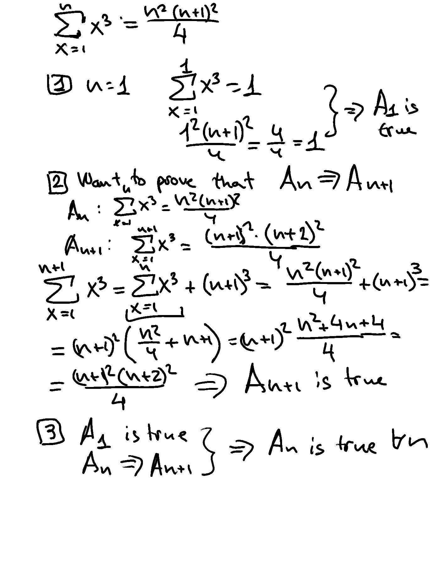
Claim: $\sum\limits^{n}_{x = 1} x^3 = \frac{n^2(n+1)^2}{4}$. We will prove this claim by induction.

Step one: P(1) is true. Consider the case where $n = 1$.

Note that $\sum\limits_{x = 1}^1 x^3 = 1^3 = 1$.
Note also that

\[\begin{split} \begin{align*} \frac{n^2 (n + 1)^2}{4} &= \frac{1^2 (1 + 1)^2}{4} \\ &= \frac{1 (2)^2}{4} \\ &= \frac{1 (4)}{4} \\ &= \frac{4}{4} \\ &= 1 \end{align*} \end{split}\]

Thus the claim is true when $n = 1$.

Step two: $P(k)$ true implies $P(k+1)$ true. Suppose that the claim is true when $n = k$, so that

\[\sum_{x = 1}^k x^3 = \frac{k^2 (k + 1)^2}{4}\]

Consider the case where $n = (k + 1)$. We have

\[\begin{split} \begin{align*} \sum_{x = 1}^{k + 1} x^3 &= \left( \sum_{x =1}^k x^3 \right) + (k + 1)^3 \\ &= \frac{k^2 (k + 1)^2}{4} + (k + 1)^3 \text{ from the inductive assumption } \\ &= \frac{k^2 (k + 1)^2}{4} + \frac{4 (k + 1)^3}{4} \\ &= \frac{k^2 (k + 1)^2 + 4 (k + 1)^3}{4} \\ &= \frac{(k + 1)^2 \{ k^2 + 4 (k + 1) \}}{4} \\ &= \frac{(k + 1)^2 \{ k^2 + 4k + 4 \}}{4} \\ &= \frac{(k + 1)^2 (k + 2)^2}{4} \\ &= \frac{(k + 1)^2 ((k + 1) + 1)^2}{4} \end{align*} \end{split}\]

Thus we have

\[\sum_{ x = 1}^n x^3 = \frac{n^2 (n + 1)^2}{4}\]

As such, we know that $P(k)$ implies $P(k + 1)$.

Step three: Conclusion

We have shown that the claim is true for the case where $n = (k + 1)$ if it is true for the case where $n = k$. We have also shown that the claim is true for the case where $n = 1$. Thus we know, from the principle of mathematical induction, that the claim is true for all $n \in \mathbb{N}$.

Example

Claim: $\sum^n_{x = 1} (2x − 1) = n^2$

We will prove this claim by induction.

Step one: P(1) is true. Consider the case where $n = 1$.

Note that $\sum_{x = 1}^{1} (2x − 1) = 2 (1) − 1 = 2 − 1 = 1$

and $1^2 = 1$. Thus the claim is true when $n = 1$.

Step two: $P(k)$ true implies $P(k+1)$ true. Suppose that the claim is true when $n = k$, so that

\[\sum^k_{x = 1} (2x − 1) = k^2\]

Consider the case where $n = (k + 1)$. We have

\[\begin{split} \begin{align*} \sum_{x = 1}^{k + 1} (2x − 1) \\ &= \left( \sum_{x =1}^k (2x − 1) \right) + (2 (k + 1) − 1) \\ &= k^2 + (2 (k + 1) − 1) \text{ from the inductive assumption } \\ &= k^2 + (2k + 2 − 1) \\ &= k^2 + (2k + 1) \\ &= k2 + 2k + 1 \\ &= (k + 1)^2 \end{align*} \end{split}\]

Thus we have

\[\sum_{x = 1}^{k + 1} (2x − 1) = (k + 1)^2\]

As such, we know that $P(k)$ implies $P(k + 1)$.

Step three: Conclusion

We have shown that the claim is true for the case where $n = (k + 1)$ if it is true for the case where $n = k$. We have also shown that the claim is true for the case where $n = 1$. Thus we know, from the principle of mathematical induction, that the claim is true for all $n \in \mathbb{N}$.

Example

We want to show that $n < 2^n$ for all $n \in \mathbb{N}$. The proof proceeds as follows:

Note that $1 < 2^1 = 2$, so the claim is true when $n = 1$.
Assume that the claim is true when $n = k$. This means that $k < 2^k$.
Consider the case of $n = (k + 1)$.
If we add $1$ to both sides of the inequality in our inductive assumption, we obtain $k + 1 < 2^k + 1$.
Since $k \geqslant 1$, we know that $1 < 2 = 2^1 \leqslant 2^k$.
This means that $1 \leqslant 2^k$.
This means that $2^k + 1 < 2^k + 2^k$.
Note that $2^k + 2^k = 2(2^k ) = 2^{k+1}$.
This means that $2^k + 1 < 2^{k+1}$.
Since $k + 1 < 2^k + 1$ and $2^k + 1 < 2^{k+1}$, we know that $(k + 1) < 2^{k+1}$.
Thus, if the proposition is true when $n = k$, then it must also be true when $n = (k + 1)$.
Since (a) the claim is true for $n = 1$, and (b) the claim is true for $n = k$, then it is also true for $n = (k + 1)$, we can conclude, by the principle of mathematical induction, that the claim is true for all $n \in \mathbb{N}$.

This example comes from Exercise A.1.7 in [Simon and Blume, 1994] (p. 858).

Arithmetic progressions#

Consider a real sequence $\{ x_n \}_{n \in \mathbb{N}}$ in which $x_n = a + (n − 1) d$.

This sequence is known as an arithmetic progression because the difference between any two consecutive terms of the sequence (with the highest index first: $x_{m+1} − x_m$) is equal to $d$.

The infinite series associated with this sequence is

\[ \sum_{n=1}^\infty (a + (n − 1) d ) = \sum_{k=0}^\infty (a + kd)\]

The partial sum of the first (N + 1) terms of this series is given by

\[\begin{split} \begin{align*} S_{(N+1)} &= \sum_{n=1}^{N + 1} (a + (n − 1) d ) \\ &= \sum_{k=0}^{N} (a + kd ) \\ &= \frac{(2a + Nd ) (N + 1)}{2} \end{align*} \end{split}\]

This validity of this formula can be established through a proof by induction. We do this below (after some other brief comments).

Note that the partial sum of the first $N$ terms of an arithmetic progression is given by

\[S_N = \frac{(2a + (N − 1)d ) N}{2} = (N) \left( \frac{\{ (a) + (a + (N − 1) d ) \}}{2} \right)\]

As is noted in [Shannon, 1995] (p. 302), this formula has a very simple interpretation. It is simply the number of terms in the sequence that are being summed times the average of the first and last terms in that sequence.

Fact

$\sum\limits^{N+1}_{n=1} (a + (n − 1) d ) = \frac{(2a+Nd )(N+1)}{2}$.

Proof

Note that the following proof is based on the one that is provided in [Basov, 2011] (pp. 22-23). By mathematical induction on $N$.

Let $N = 1$. We have

\[\begin{split} \sum_{n=1}^{N + 1} (a + (n − 1) d ) = \sum_{n=1}^2 (a + (n − 1) d ) \\ = (a + (1 − 1)d ) + (a + (2 − 1)d ) \\ = (a + 0d + a + 1d ) \\ = (2a + d ) \end{split}\]

and

\[ \frac{(2a + Nd ) (N + 1)}{2} = \frac{(2a + 1d ) (1 + 1)}{2} = \frac{(2a + d )(2)}{2} = (2a + d )\]

Thus the claim is true for $N = 1$.

Assume that the claim is true for $N = k$. In other words, assume that

\[ \sum_{n=1}^{k + 1} (a + (n − 1) d ) = \frac{(2a + kd ) (k + 1)}{2}\]

(Call this the “inductive assumption”.)

Now consider the case when $N = (k + 1)$. We have

\[\begin{split} \begin{align*} \sum_{n=1}^{k + 2} (a + (n − 1) d ) \\ &= \left( \sum_{n=1}^{k + 1} (a + (n − 1) d ) \right) + (a + (k + 2 − 1) d ) \\ &= \frac{(2a + kd ) (k + 1)}{2} + (a + (k + 1)d ) \text{ (by the inductive assumption) } \\ &= \frac{(2a + kd ) (k + 1)}{2} + \frac{(2a + 2(k + 1)d )}{2} \\ &= \frac{2a(k + 1) + k(k + 1)d + 2a + 2(k + 1)d}{2} \\ &= \frac{2a ((k + 1) + 1) + ((k + 1) + 1) (k + 1)d}{2} \\ &= \frac{(2a + (k + 1)d ) ((k + 1) + 1)}{2} \end{align*} \end{split}\]

Since this is in the required form, and we used the inductive assumption in the process of deriving it, we have shown that, if the claim is true when $N = k$, then it is also true when $N = (k + 1)$.

Since $P(1)$ is true, and $P(k) \Rightarrow P(k + 1)$, we know, by the principle of mathematical induction, that the claim is true for all $N \in \mathbb{N}$.

Note that the sum of all of the terms in an infinite arithmetic progression is unbounded, since

\[\begin{split} \begin{align*} S_\infty &= \lim_{N \rightarrow \infty} S_{N + 1} \\ &= \lim_{N \rightarrow \infty} \sum_{n=1}^{N + 1} (a + (n − 1)d ) \\ &= \lim_{N \rightarrow \infty} \frac{(2a + Nd ) (N + 1)}{2} \\ &= \begin{cases} \infty \quad \text{ if } d > 0, \\ −\infty \quad \text{ if } d < 0. \end{cases} \end{align*} \end{split}\]

Geometric progressions#

Consider a real sequence $\{ x_n \}_{n \in \mathbb{N}}$ in which $x_n = ar^{(n−1)}$. We will assume that $r \notin \{ 0, 1 \}$.

This sequence is known as a geometric progression because the ratio of any two consecutive terms of the sequence (with the highest index on numerator: $\frac{x_{m+1}}{x_m}$ ) is equal to $r$.

The infinite series associated with this sequence is

\[ \sum_{n=1}^{\infty} ar^{(n−1)} = \sum_{k=0}^{\infty} ar^k\]

The partial sum of the first $(N + 1)$ terms of this series is given by

\[\begin{split} \begin{align*} S_{(N+1)} &= \sum_{n=1}^{N+1} ar^{(n−1)} \\ &= \sum_{k=0}^{N} ar^k \\ &= a \sum_{k=0}^N r^k \\ &= \frac{a ( 1 − r^{(N+1)})}{(1 − r )} \end{align*} \end{split}\]

This validity of this formula can be established through a proof by induction. This is left for you to do as an exercise.

The sum of all of the terms in an infinite geometric progression is given by

\[\begin{split} \begin{align*} S_\infty &= \lim_{N \rightarrow \infty} S_{N+1} \\ &= \lim_{N \rightarrow \infty} \sum_{n=1}^{N+1} ar^{(n−1)} \\ &= \lim_{N \rightarrow \infty} \frac{a ( 1 − r^{(N+1)})}{(1 − r )} \\ &= \begin{cases} \frac{a}{(1−r )} \quad \text{ if } |r| < 1, \\ \pm\infty \quad \text{ if } |r| > 1. \end{cases} \end{align*} \end{split}\]

Application: financial economics#

In economics, finance, and accounting, we often need to evaluate time streams of payoffs.
In general, we cannot simply add them all together in their raw form.
There are many reasons for this. Some of these reasons include the following:
- Inflation (or deflation): The purchasing power of one dollar varies over time.
- Foregone interest: There is an opportunity cost of time in the form of interest that could be earned.
- Time preference: People might have a preference for the timing of payoffs.
We need to adjust the raw payoffs to put them in a commensurable form.
This might involve using constant dollar estimates or accounting for expected inflation to deal with changes in the price level.
It might involve calculating the present value (or a specific period future value) of all of the payoffs.
It might involve discounting future payoffs in some fashion if the decision-maker is impatient.
The techniques for doing this are part of the subject matter of decision theory (from microeconomics) and financial mathematics.
The mathematical techniques that are employed in financial mathematics include sequences, series, limits, and polynomial equations.

Overview of this application:

Simple interest
Compound interest
Present value and future value

Simple interest#

Suppose that you borrow $P$ now (period zero) and are required to pay it off in one single payment in period $n$.
You will be charged simple interest at the rate of $100 (i )$ per cent per period.
Simple interest is only charged on the remaining principal at a point in time and not on the entire balance owed at that point in time.
If you do not make any payments on the loan until the end of the loan, the sequence of additions to your loan balance is $\{ At \}^n_{t=0} = \{ P, iP, iP, \dots , iP \}$.
If you do not make any payments on the loan until the end of the loan, the sequence of outstanding loan balances is $\{ Bt \}^n_{t=0} = \{ P, P + iP, P + 2iP, \dots , P + niP \}$. (Note that this is an arithmetic progression. However, this does not really matter here, because we do not need to calculate its sum.)
If no repayments are made until period n and the entire outstanding balance is repaid in that period, the future amount that must be paid in period $n$ is given by

\[ S_n = P + \sum_{k=1}^n iP = P + niP = (1 + ni ) P\]

In this case, the total interest payments on this loan are equal to

\[ I_S = S_n − P = (1 + ni ) P − P = niP \]

Compound interest#

Suppose that you borrow $P$ now (period zero) and are required to pay it off in one single payment in period $n$.
You will be charged compound interest at the rate of $100 (i )$ per cent per period.
Compound interest is charged on the entire balance owed at a point in time.
The compounding will take place once per period, so that the compounding periods and the charging periods coincide.
If you do not make any payments on the loan until the end of the loan, the sequence of additions to your loan balance is $ \{ At \}^n_{t=0} = \{ P, iP, i (1 + i )P, \dots , i (1 + i )^{(n−1)}P \}$.
If you do not make any payments on the loan until the end of the loan, the sequence of outstanding loan balances is $\{ Bt \}^n_{t=0} = \{ P, (1 + i )P, (1 + i )^2 P, \dots , (1 + i )^n P \}$. (Note that this is a geometric progression. However, this does not really matter here, because we do not need to calculate its sum.)
How do we get this sequence of balances? If your balance in period $(n − 1)$ is $(1 + i )^{(n−1)}P$, then you will be charged $iB_{(n−1)} = i(1 + i )^{(n−1)}P$ in interest. This will be added to your balance. Thus your new balance in period n will be

\[B_{(n−1)} + iB_{(n−1)} = (1 + i )B+{(n−1)} = (1 + i )(1 + i )^{(n−1)}P = (1 + i )^n P\]

Another way to think about the future amount that must be paid in period $n$ (that is, the balance in period $n$) is as follows.

\[ S_n = S_{n−1} + iS_{n−1} = (1 + i ) S+{n−1} \]

This means that

\[\begin{split} \begin{align*} S_n &= (1 + i ) S+{n−1} \\ &= (1 + i ) (1 + i ) S_{n−2} \\ &= (1 + i )^2 S_{n−2} \\ &= \dots \\ &= (1 + i )^n S_{n−n} \\ &= (1 + i )^n S_0 \end{align*} \end{split}\]

Since $S_0 = P$, we have $S_n = (1 + i)^n P$.

Thus the total interest payments are equal to

\[ I_C = S_n − P = (1 + i )^n P − P = \{(1 + i )^n − 1\} P\]

Present and future values#

We will often be interested in calculating the present value or future value of a payment stream. Suppose that we have a sequence of $(n + 1)$ payments given by $\{ P_0, P_1, P_2, \dots , P_n \}$.

Suppose also that the expected per-period interest rate is believed to be constant over the entire length of time that is covered by this payment sequence. This interest rate is given by $r \in (0, 1)$. (Note that $r \in (0, 1)$ simply means that $0 < r < 1$.)

If you invest $1 in period $t$, you will expect to recieve $$1(1 + r)$ in period $(t + 1)$. Applying this logic and the principle of compounding, we can obtain the future value of this payment stream. We will assume that the compounding period is the same as the payment period.

The future value of this payment stream is

\[\begin{split} S_n = \sum_{t=0}^n P_t (1 + r )^{n−t} \\ = P_0 (1 + r )^{n−0} + P_1 (1 + r )^{n−1} + P_2 (1 + r )^{n−2} + \dots + P_n (1 + r )^{n−n} \\ = P_0 (1 + r )^{n} + P_1 (1 + r )^{n−1} + P_2 (1 + r )^{n−2} + \dots + P_n (1 + r )^{0} \\ = P_0 (1 + r )^{n} + P_1 (1 + r )^{n−1} + P_2 (1 + r )^{n−2} + \dots + P_n (1) \\ = P_0 (1 + r )^{n} + P_1 (1 + r )^{n−1} + P_2 (1 + r )^{n−2} + \dots + P_n \end{split}\]

The present value of the payment stream is simply the amount that you would need to invest now to receive this future value in the presence of compounding without making any further deposits. As before, we will assume that the compounding period is the same as the payment period. The present value of this payment stream is given by:

\[\begin{split} \begin{align*} S_0 &= \frac{S_n}{(1 + r )^n} \\ &= \left( \frac{1}{(1 + r )^n} \right) \left( \sum_{t=0}^n P_t (1 + r )^{n−t} \right) \\ &= \sum_{t=0}^n P_t \frac{(1 + r )^{n−t}}{(1 + r )^n} \\ &= \sum_{t=0}^n \frac{P_t}{(1 + r)^t} \end{align*} \end{split}\]

Note that the present value of this payment stream can be written as

\[\begin{split} S_0 = \sum_{t=0}^n \frac{P_t}{(1 + r )^t} \\ = \frac{P_0}{(1 + r )^0} + \frac{P_1}{(1 + r )^1} + \frac{P_2}{(1 + r)^2} + \dots + \frac{P_n}{(1 + r )^n} \\ = \frac{P_0}{1} + \frac{P_1}{(1 + r )^1} + \frac{P_2}{(1 + r)^2} + \dots + \frac{P_n}{(1 + r )^n} \\ = P_0 + \frac{P_1}{(1 + r )^1} + \frac{P_2}{(1 + r)^2} + \dots + \frac{P_n}{(1 + r )^n} \end{split}\]

Identical payments#

Suppose that you receive a constant stream of $(n + 1)$ payments (or, rather, a stream of constant payments) of the form $\{ P_0, P_1, P_2, \dots , P_n \} = \{ A, A, A, \dots , A \}$.

These types of payment streams, along with some variations, are known as “annuities”.

In future value terms, this stream of payments is

\[\begin{split} \{ P^n_0 , P^n_1 , P^n_2 , \dots , P^n_n \} \\ = \{ A (1 + r )^n , A (1 + r )^{n−1} , A (1 + r )^{n−2} , \dots , A \}\end{split}\]

Note that this is a geometric progression in which $a = A$, “r” $= q = (1 + r )$, and there are $(n + 1)$ terms.

In present value terms, this stream of payments is

\[\begin{split} \{ P^0_0, P^0_1 , P^0_2, \dots , P^0_n \} \\ = \left\{ A, \frac{A}{(1 + r )} , \frac{A}{(1 + r )^2} , \dots , \frac{A}{(1 + r)^n} \right\} \\ = \{ A, A (1 + r)^{−1} , A (1 + r)^{−2} , \dots , A (1 + r )^{−n} \} \end{split}\]

Note that this is a geometric progression in which $a = A$, “r”$ = q = \frac{1}{(1+r )} = (1 + r )^{−1}$, and there are $(n + 1)$ terms.

The future value of this stream of payments is

\[\begin{split} \begin{align*} S_n &= \sum_{t=0}^n P_t (1 + r)^{n−t} \\ &= \sum_{t=0}^n A (1 + r )^{n−t} \\ &= \frac{A ( 1 − (1 + r )^{n+1})}{1 − (1 + r )} \\ &= \frac{A ( 1 − (1 + r )^{n+1})}{1 − 1 - r } \\ &= \frac{A ( 1 − (1 + r )^{n+1})}{- r } \\ &= \frac{A ( (1 + r )^{n+1} + 1)}{ r } \\ \end{align*} \end{split}\]

The present value of this stream of payments is

\[\begin{split} \begin{align*} S_0 &= \sum_{t=0}^n \frac{P_t}{(1 + r )^t} \\ &= \sum_{t=0}^n \frac{A}{(1 + r )^t} \\ &= \frac{A( 1 − ((1 + r )^{−1})^{n+1})}{1 − (1 + r )^{−1}} \\ &= \frac{A(1 − (1 + r )^{−(n+1)})}{( \frac{1+r}{1+r}) − ( \frac{1}{1+r})} \\ &= \frac{A(1 − (1 + r )^{−(n+1)})}{( \frac{1+r −1}{1+r})} \\ &= \frac{A(1 − (1 + r )^{−(n+1)})}{( \frac{r}{1+r})} \\ &= \frac{A(1 + r)(1 − (1 + r )^{−(n+1)})}{( r)} \end{align*} \end{split}\]

Note that

\[\begin{split} \begin{align*} \frac{S_n}{(1 + r )^n} &= \left( \frac{1}{(1 + r )^n} \right) \bigg( \frac{A((1 + r )^{n+1} − 1)}{r} \bigg) \\ &= \frac{A((1 + r )^{n+1} − 1)}{r (1 + r )^n} \\ &= \frac{A((1 + r )^{n+1} − 1)(1 + r )^{−n}}{r} \\ &= \frac{A((1 + r )^{n+1−n} − (1 + r ){−n})}{r} \\ &= \frac{A((1 + r ) − (1 + r )^{−n})}{r} \\ &= \frac{A (1 + r )( 1 − (1 + r )^{−(n+1)})}{r} \\ &= S_0 \end{align*} \end{split}\]

Types of Annuities#

There are many types of annuities. Using the terminology that is employed by [Shannon, 1995], these include the following:

Ordinary annuity: Payment periods and compounding periods coincide, payments begin in the next period (or, equivalently, at the “end” of this period).
Ordinary annuity due: Payment periods and compounding periods coincide, payments begin in the current period (or, equivalently, at the “beginning” of this period).
General annuities: Payment periods and compounding periods differ. (These may occur in both annuity and annuity due form.)
Perpetuities: An annuity in which there are an infinite number of payment periods. (These may occur in both annuity and annuity due form. They may also occur in both ordinary and general form.)

Notes from the lecture#

Hand written notes from the lecture

📖 Sequences, series and convergence

Contents

📖 Sequences, series and convergence#

Sources and reading guide#

Sequences#

Convergence and limit#

Properties of limits#

Cauchy sequences#

Sub-sequences#

Mathematical application: Euler’s constant (\(e\))#

Series#

Proof by mathematical induction#

Arithmetic progressions#

Geometric progressions#

Application: financial economics#

Simple interest#

Compound interest#

Present and future values#

Identical payments#

Types of Annuities#

Notes from the lecture#